So far we’ve used CGrateS to rate a basic CDR and get a cost for it, but in the real world, we’d usually associate the cost with an account, which would represent a business or a person, who will ultimately be charged for using the service.
Note: I’ve put the code for all this in Github, if you’ve got issues following along, or don’t want to copy and paste the code from the website, you can grab the code here.
Creating an Account
Let’s start off by creating an account inside CGrateS – This is kinda pointless, but we’ll talk more about that later:
#Create the Account object inside CGrateS
Create_Account_JSON = {
    "method": "ApierV2.SetAccount",
    "params": [
        {
            "Tenant": "cgrates.org",
            "Account": "Nick_Test_123"
        }
    ]
}
print(CGRateS_Obj.SendData(Create_Account_JSON))
Running this onto the API should create an account named “Nick_Test_123”, but let’s confirm that’s the case:
#Print the Account Information
pprint.pprint(CGRateS_Obj.SendData({'method':'ApierV2.GetAccount','params':[{"Tenant":"cgrates.org","Account": "Nick_Test_123"}]}))
Running this will give us the information about the account we just created:
{'method': 'ApierV2.GetAccount', 'params': [{'Tenant': 'cgrates.org', 'Account': 'Nick_Test_123'}]}
OrderedDict([('id', None),
             ('result',
              OrderedDict([('ID', 'cgrates.org:Nick_Test_123'),
                           ('BalanceMap', None),
                           ('UnitCounters', None),
                           ('ActionTriggers', None),
                           ('AllowNegative', False),
                           ('Disabled', False),
                           ('UpdateTime',
                            '2023-10-09T16:53:37.524466041+11:00')])),
             ('error', None)])
That was easy!
There’s not really much to see on our account at this stage, other than the UpdateTime, there’s nothing really going on, we don’t have any Balances.
Adding Balance for Voice
Accounts exist for spending, so let’s add a balance to this account to send from.
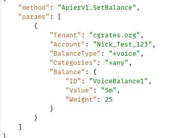
We’ll use the SetBalance API to create a new balance with 5 minutes of talk time, that we can use for making a call, and talking, for (you guessed it) – 5 minutes, so and we’ll use the balance “5_minute_voice_balance” that we’ll create:
#Add a balance to the account with type *voice with 5 minutes of Talk Time
Create_Voice_Balance_JSON = {
    "method": "ApierV1.SetBalance",
    "params": [
        {
            "Tenant": "cgrates.org",
            "Account": "Nick_Test_123",
            "BalanceType": "*voice",
            "Categories": "*any",
            "Balance": {
                "ID": "5_minute_voice_balance",
                "Value": "5m",
                "Weight": 25
            }
        }
    ]
}
print(CGRateS_Obj.SendData(Create_Voice_Balance_JSON))
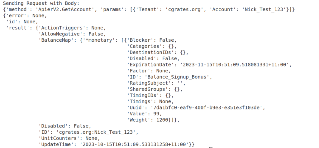
Now if we run the GetAccount API command again, we should see the new balance we just created:
#Print the Account Information
pprint.pprint(CGRateS_Obj.SendData({'method':'ApierV2.GetAccount','params':[{"Tenant":"cgrates.org","Account": "Nick_Test_123"}]}))
{'method': 'ApierV2.GetAccount', 'params': [{'Tenant': 'cgrates.org', 'Account': 'Nick_Test_123'}]}
{'error': None,
 'id': None,
 'result': {'ActionTriggers': None,
            'AllowNegative': False,
            'BalanceMap': {'*voice': [{'Blocker': False,
                                       'Categories': None,
                                       'DestinationIDs': None,
                                       'Disabled': False,
                                       'ExpirationDate': '0001-01-01T00:00:00Z',
                                       'Factor': None,
                                       'ID': '5_minute_voice_balance',
                                       'RatingSubject': '',
                                       'SharedGroups': None,
                                       'TimingIDs': None,
                                       'Timings': None,
                                       'Uuid': '37423d07-d99a-40b1-851a-981c3df02cb3',
                                       'Value': 300000000000,
                                       'Weight': 25}]},
            'Disabled': False,
            'ID': 'cgrates.org:Nick_Test_123',
            'UnitCounters': None,
            'UpdateTime': '2023-10-14T17:58:23.801531205+11:00'}}
So now we’ve got a new balance named ‘5_minute_voice_balance‘:
- The type is *voice, because this balance is storing talk time
- The weight of this balance is 25, this means this balance should take priority over any balances with a lower value than 25 (that’s right, we can (and will) do tiered balances)
- The value is 300000000000 nanoseconds, which equates to 5 minutes (yes, that’s the correct number of zeros)
Okay, but Nick_Test_123 probably wants to make some calls, so let’s generate a 2.5 minute call event and check out what happens.
#Generate a new call event for a 2.5 minute (150 second) call
Process_External_CDR_JSON = {
    "method": "CDRsV2.ProcessExternalCDR",
    "params": [
        {
            "OriginID": str(uuid.uuid1()),
            "ToR": "*voice",
            "RequestType": "*pseudoprepaid",
            "AnswerTime": now.strftime("%Y-%m-%d %H:%M:%S"),
            "SetupTime": now.strftime("%Y-%m-%d %H:%M:%S"),
            "Tenant": "cgrates.org",
            "Account": "Nick_Test_123",
            "Usage": "150s",
        }
    ]
}
print(CGRateS_Obj.SendData(Process_External_CDR_JSON))
Alright, now we’ve got a call event, let’s call the GetAccount API again to check the balance:
#Print the Account Information
pprint.pprint(CGRateS_Obj.SendData({'method':'ApierV2.GetAccount','params':[{"Tenant":"cgrates.org","Account": "Nick_Test_123"}]}))
{'method': 'ApierV2.GetAccount', 'params': [{'Tenant': 'cgrates.org', 'Account': 'Nick_Test_123'}]}
{'error': None,
 'id': None,
 'result': {'ActionTriggers': None,
            'AllowNegative': False,
            'BalanceMap': {'*voice': [{'Blocker': False,
                                       'Categories': None,
                                       'DestinationIDs': None,
                                       'Disabled': False,
                                       'ExpirationDate': '0001-01-01T00:00:00Z',
                                       'Factor': None,
                                       'ID': '5_minute_voice_balance',
                                       'RatingSubject': '',
                                       'SharedGroups': None,
                                       'TimingIDs': None,
                                       'Timings': None,
                                       'Uuid': '37423d07-d99a-40b1-851a-981c3df02cb3',
                                       'Value': 150000000000,
                                       'Weight': 25}]},
            'Disabled': False,
            'ID': 'cgrates.org:Nick_Test_123',
            'UnitCounters': None,
            'UpdateTime': '2023-10-14T17:58:23.80925546+11:00'}}
And there you have it, we’ve used 150 seconds of our 300 second (5 minutes) of talk time in this balance, leaving with us 150000000000 nanoseconds (150 seconds) remaining!
And with that progress, now is a great time to pause and talk about some theory that’s really important to grasp!
Balance Types
But *voice is just one balance type – We can support multiple balance types; we’ve just given a balance of *voice for talk time, but we could also give a credit to the balance for *sms or *data, you name it (*generic) and cash (*monetary) and we can have multiple separate balances for each.
This means we can have one account with something like:
- 100 minutes of Local / National Calls (Expires at the end of the month)
- 40 minutes of Mobile Calls (Expires 24 hours after it’s been created)
- 80 minutes of Mobile Calls (During “Happy Hour” from 6 to 7pm)
- 50 minutes of International Calls (Expires in 30 days)
And not just voice balance, the same account could also have:
- 1GB of Data usage
- 50 SMS to on-net destinations
- $200 of Cash (expiring never)
Phew! That’s a lot of balances, but we can do it all through CGrateS!
What Balance to Use
So if we’ve got a stack of balances defined, how does CGrateS know what balance to use?
Firstly CGrateS is going to evaluate the BalanceType, this is set on events, so if we get an event for *data CGrateS will check out the balances available for *data, and evaluate the balances by Weight, with the highest weight evaluated first.
If we get to the end of all the available balances for that BalanceType, CGrateS then evaluates *generic and then *monetary balances, again, ordered by Weight.
We can set what balance gets used based on the Destination; using DestinationIDs we can filter the Balance to only apply for calls to Local/National numbers, so a call to an International destination won’t use that balance.
We can also set an Expiry on the Balance, for example we can give a customer 30 days to use the balance, after which it expires and can’t be used, likewise we can set Timings so enable scenarios like a “Happy hour” with extra calls between 6pm and 7pm.
When we define a balance we can also set the Blocker flag to True, if this is set, it means CGrateS will not look evaluate any balances after reaching that balance.
Adding a Balance for Local / National & Mobile Calls
Let’s jump back into the practice, and define two new Balances; one for Local/National calls, and another for Mobile calls.
But first we’ll need to know what destinations are mobiles and what are local/national (fixed). We’ve covered setting Destinations previously, so let’s set up the Destinations:
CGRateS_Obj.SendData({'method':'ApierV2.SetTPDestination','params':[{"TPid":"cgrates.org","ID":"Dest_AU_Fixed","Prefixes":["612", "613", "617", "618"]}]})
CGRateS_Obj.SendData({'method':'ApierV2.SetTPDestination','params':[{"TPid":"cgrates.org","ID":"Dest_AU_Mobile","Prefixes":["614"]}]})
CGRateS_Obj.SendData({'method':'ApierV2.SetTPDestination','params':[{"TPid":"cgrates.org","ID":"Dest_AU_TollFree","Prefixes":["6113", "6118"]}]})
#Load TariffPlan we just defiend from StorDB to DataDB
print(CGRateS_Obj.SendData({"method":"APIerSv1.LoadTariffPlanFromStorDb","params":[{"TPid":"cgrates.org","DryRun":False,"Validate":True,"APIOpts":None,"Caching":None}],"id":0}))
Alright, now let’s add a balance for our local/national (fixed) calls.
To do this, we’ll add two new balances, but we’ll need to differentiate this from the 5_minute_voice_balance we created earlier, and to achieve this we weill:
- Set a higher Weight value than we have set on 5_minute_voice_balance (25) so this balance will get consumed before 5_minute_voice_balance does
- Set the DestinationIDs to match the destinations (Dest_AU_Mobile for Mobile and Dest_AU_Fixed for Local/National) we want the balance to apply to
ProTip: When you we create our Balance we can set what Destinations we want to use this balance for, if you want to specify multiple balances, we can do it by setting the Balance names as a string delimited by semicolons, like “DestinationIDs”: “Dest_AU_Fixed;Dest_AU_Mobile;Dest_AU_TollFree”
We’ll also set a balance expiry, which we’ll cover shortly, but now let’s define out 100 minutes for Local/National expiring at the end of the month:
#Add a balance to the account with type *voice with 100 minutes of talk time to Local / National Destinations expiring at the end of the month
Create_Local_National_Voice_Balance_JSON = {
    "method": "ApierV1.SetBalance",
    "params": [
        {
            "Tenant": "cgrates.org",
            "Account": "Nick_Test_123",
            "BalanceType": "*voice",
            "Categories": "*any",
            "Balance": {
                "ID": "Local_National_100_minutes_voice_balance",
                "Value": "100m",
                "ExpiryTime": "*month_end",
                "Weight": 60,
                "DestinationIDs": "Dest_AU_Fixed",
            }
        }
    ]
}
print(CGRateS_Obj.SendData(Create_Local_National_Voice_Balance_JSON))
We’ll also add our 24 hours to use to use 40 minutes of talk to mobiles, and a GetAccount to check the result:
#Add a balance to the account with type *voice with 40 minutes of talk time to Mobile Destinations expiring in 24 hours
Create_Mobile_Voice_Balance_JSON = {
    "method": "ApierV1.SetBalance",
    "params": [
        {
            "Tenant": "cgrates.org",
            "Account": "Nick_Test_123",
            "BalanceType": "*voice",
            "Categories": "*any",
            "Balance": {
                "ID": "Mobile_40_minutes_voice_balance",
                "Value": "40m",
                "ExpiryTime": "*daily",
                "Weight": 60,
                "DestinationIDs": "Dest_AU_Mobile",
            }
        }
    ]
}
print(CGRateS_Obj.SendData(Create_Mobile_Voice_Balance_JSON))

# Get Account Info Again
pprint.pprint(CGRateS_Obj.SendData({"method": "ApierV2.GetAccount", "params": [
              {"Tenant": "cgrates.org", "Account": "Nick_Test_123"}]}))
Alright, let’s try running that:
{'method': 'ApierV2.GetAccount', 'params': [{'Tenant': 'cgrates.org', 'Account': 'Nick_Test_123'}]}
{'error': None,
 'id': None,
 'result': {'ActionTriggers': None,
            'AllowNegative': False,
            'BalanceMap': {'*voice': [{'Blocker': False,
                                       'Categories': None,
                                       'DestinationIDs': None,
                                       'Disabled': False,
                                       'ExpirationDate': '0001-01-01T00:00:00Z',
                                       'Factor': None,
                                       'ID': '5_minute_voice_balance',
                                       'RatingSubject': '',
                                       'SharedGroups': None,
                                       'TimingIDs': None,
                                       'Timings': None,
                                       'Uuid': 'ad9d8bdd-64df-430f-af9d-3fc0410fd16b',
                                       'Value': 150000000000,
                                       'Weight': 25},
                                      {'Blocker': False,
                                       'Categories': None,
                                       'DestinationIDs': {'Dest_AU_Fixed': True},
                                       'Disabled': False,
                                       'ExpirationDate': '2023-10-31T23:59:59+11:00',
                                       'Factor': None,
                                       'ID': 'Local_National_100_minutes_voice_balance',
                                       'RatingSubject': '',
                                       'SharedGroups': None,
                                       'TimingIDs': None,
                                       'Timings': None,
                                       'Uuid': 'e4a2c211-8112-4e40-b3e6-250863404cc9',
                                       'Value': 6000000000000,
                                       'Weight': 60},
                                      {'Blocker': False,
                                       'Categories': None,
                                       'DestinationIDs': {'Dest_AU_Mobile': True},
                                       'Disabled': False,
                                       'ExpirationDate': '2023-10-15T18:15:11.521636734+11:00',
                                       'Factor': None,
                                       'ID': 'Mobile_40_minutes_voice_balance',
                                       'RatingSubject': '',
                                       'SharedGroups': None,
                                       'TimingIDs': None,
                                       'Timings': None,
                                       'Uuid': 'd4cbf6d8-50a5-4c97-82c2-dfe9936ae8d1',
                                       'Value': 2400000000000,
                                       'Weight': 60}]},
            'Disabled': False,
            'ID': 'cgrates.org:Nick_Test_123',
            'UnitCounters': None,
            'UpdateTime': '2023-10-14T18:15:11.524242437+11:00'}}
Alright! We now have 3 balances defined!
Notice in the API in the expiry I put *daily and *month_end, but in the output it’s got a real date and time (I wrote this 14/10/23 around 07:00 UTC, hence why those dates are what they are).
I could have specified the date and time in the API of a specific time I wanted the balance to expire (You can too, just replace “*daily” with “2024-01-01T00:00:00Z” for example), but that’s a pain in the butt, especially considering most of the time these values will be something common.
The *month_end is a special “meta” value, there’s a heap of these that allow us to do things like “current time + 20 minutes” (+20m), this time next month (*monthly), “this time tomorrow” (*daily), or “this time next week” (+168h) – You can find the full list of special dates here.
From a product perspective, setting an expiry on balances means we can set credit to expire 2 years after the subscriber tops up, but the same logic can be used so a subscriber could purchase a 7 day addon pack, that expires in 7 days, or a monthly plan can automatically expire in 30 days.
Now if we call the ProcessExternalCDR API again with a call to a Mobile and a Fixed number, we’ll see the respective balances get deducted.
#Generate a new call event for a 2.5 minute (150 second) call to a mobile number
Process_External_CDR_JSON = {
    "method": "CDRsV2.ProcessExternalCDR",
    "params": [
        {
            "OriginID": str(uuid.uuid1()),
            "ToR": "*voice",
            "RequestType": "*pseudoprepaid",
            "AnswerTime": now.strftime("%Y-%m-%d %H:%M:%S"),
            "SetupTime": now.strftime("%Y-%m-%d %H:%M:%S"),
            "Subject": "61412341234",
            "Destination": "61412341234",
            "Tenant": "cgrates.org",
            "Account": "Nick_Test_123",
            "Usage": "30s",
        }
    ]
}
print(CGRateS_Obj.SendData(Process_External_CDR_JSON))

#Generate a new call event for a 2.5 minute (150 second) call to a fixed line local/national number
Process_External_CDR_JSON = {
    "method": "CDRsV2.ProcessExternalCDR",
    "params": [
        {
            "OriginID": str(uuid.uuid1()),
            "ToR": "*voice",
            "RequestType": "*pseudoprepaid",
            "AnswerTime": now.strftime("%Y-%m-%d %H:%M:%S"),
            "SetupTime": now.strftime("%Y-%m-%d %H:%M:%S"),
            "Subject": "61212341234",
            "Destination": "61212341234",
            "Tenant": "cgrates.org",
            "Account": "Nick_Test_123",
            "Usage": "30s",
        }
    ]
}
print(CGRateS_Obj.SendData(Process_External_CDR_JSON))

# Get Account Info Again
pprint.pprint(CGRateS_Obj.SendData({"method": "ApierV2.GetAccount", "params": [
              {"Tenant": "cgrates.org", "Account": "Nick_Test_123"}]}))
We should see the minutes reduced by 30 seconds for our Local_National_100_minutes_voice_balance and Mobile_40_minutes_voice_balance balances, while our 5_minute_voice_balance hasn’t been touched.
{
   "Blocker":false,
   "Categories":"None",
   "DestinationIDs":"None",
   "Disabled":false,
   "ExpirationDate":"0001-01-01T00:00:00Z",
   "Factor":"None",
   "ID":"5_minute_voice_balance",
   "RatingSubject":"",
   "SharedGroups":"None",
   "TimingIDs":"None",
   "Timings":"None",
   "Uuid":"29f21735-1d62-49b1-9c53-80eab6f7b005",
   "Value":150000000000,
   "Weight":25
},
{
   "Blocker":false,
   "Categories":"None",
   "DestinationIDs":{
      "Dest_AU_Fixed":true
   },
   "Disabled":false,
   "ExpirationDate":"2023-10-31T23:59:59+11:00",
   "Factor":"None",
   "ID":"Local_National_100_minutes_voice_balance",
   "RatingSubject":"",
   "SharedGroups":"None",
   "TimingIDs":"None",
   "Timings":"None",
   "Uuid":"54db4f60-342e-4738-aaf1-a1304badc41d",
   "Value":5970000000000,
   "Weight":60
},
{
   "Blocker":false,
   "Categories":"None",
   "DestinationIDs":{
      "Dest_AU_Mobile":true
   },
   "Disabled":false,
   "ExpirationDate":"2023-10-15T18:32:34.888821482+11:00",
   "Factor":"None",
   "ID":"Mobile_40_minutes_voice_balance",
   "RatingSubject":"",
   "SharedGroups":"None",
   "TimingIDs":"None",
   "Timings":"None",
   "Uuid":"501eb00e-e947-4675-926f-080911e66897",
   "Value":2370000000000,
   "Weight":60
}
One last thing we’ll try before we end, our Mobile_40_minutes_voice_balance has still got 39.5 minutes left, and our 5_minute_voice_balance has still got minutes remaining, so if we try and make a call that’s 2450 seconds (~41 minutes), we should consume all the remaining minutes in Mobile_40_minutes_voice_balance and the go onto consume the remaining 1 minute out of 5_minute_voice_balance.
Let’s test this theory!
#Generate a new call event for a 42 minute call to a mobile to use all of our Mobile_40_minutes_voice_balance and start consuming 5_minute_voice_balance
Process_External_CDR_JSON = {
    "method": "CDRsV2.ProcessExternalCDR",
    "params": [
        {
            "OriginID": str(uuid.uuid1()),
            "ToR": "*voice",
            "RequestType": "*pseudoprepaid",
            "AnswerTime": now.strftime("%Y-%m-%d %H:%M:%S"),
            "SetupTime": now.strftime("%Y-%m-%d %H:%M:%S"),
            "Subject": "61412341234",
            "Destination": "61412341234",
            "Tenant": "cgrates.org",
            "Account": "Nick_Test_123",
            "Usage": "2450s",
        }
    ]
}
print(CGRateS_Obj.SendData(Process_External_CDR_JSON))

# Get Account Info Again
pprint.pprint(CGRateS_Obj.SendData({"method": "ApierV2.GetAccount", "params": [
              {"Tenant": "cgrates.org", "Account": "Nick_Test_123"}]}))
Let’s check the output:
{
   "Blocker":false,
   "Categories":"None",
   "DestinationIDs":"None",
   "Disabled":false,
   "ExpirationDate":"0001-01-01T00:00:00Z",
   "Factor":"None",
   "ID":"5_minute_voice_balance",
   "RatingSubject":"",
   "SharedGroups":"None",
   "TimingIDs":"None",
   "Timings":"None",
   "Uuid":"29f21735-1d62-49b1-9c53-80eab6f7b005",
   "Value":70000000000,
   "Weight":25
},
...
{
   "Blocker":false,
   "Categories":"None",
   "DestinationIDs":{
      "Dest_AU_Mobile":true
   },
   "Disabled":false,
   "ExpirationDate":"2023-10-15T18:44:18.161474861+11:00",
   "Factor":"None",
   "ID":"Mobile_40_minutes_voice_balance",
   "RatingSubject":"",
   "SharedGroups":"None",
   "TimingIDs":"None",
   "Timings":"None",
   "Uuid":"501eb00e-e947-4675-926f-080911e66897",
   "Value":0.0161939859,
   "Weight":60
}
Boom, there we have it! Used all of the minutes in Mobile_40_minutes_voice_balance and started eating into the 5_minute_voice_balance.
Note: I’ve put the code for all this in Github, if you’ve got issues following along, or don’t want to copy and paste the code from the website, you can grab the code here.
Alright, that was a long post! Sorry about that, and props for making it to the end, still so much to learn about CGrateS.
Other posts in the CGrateS in Baby Steps series: