The Binding Support Function is used in 4G and 5G networks to allow applications to authenticate against the network, it’s what we use to authenticate for XCAP and for an Entitlement Server.
Rather irritatingly, there are two BSF addresses in use:
If the ISIM is used for bootstrapping the FQDN to use is:
bsf.ims.mncXXX.mccYYY.pub.3gppnetwork.org
But if the USIM is used for bootstrapping the FQDN is
bsf.mncXXX.mccYYY.pub.3gppnetwork.org
You can override this by setting the 6FDA EF_GBANL (GBA NAF List) on the USIM or equivalent on the ISIM, however not all devices honour this from my testing.
One of the hyped benefits of a 5G Core Networks is that 5GC can be used for wired networks (think DSL or GPON) – In marketing terms this is called “Wireless Wireline Convergence” (5G WWC) meaning DSL operators, cable operators and fibre network operators can all get in on this sweet 5GC action and use this sexy 5G Core Network tech.
This is something that’s in the standards, and that the big kit vendors are pushing heavily in their marketing materials. But will it take off? And should operators of wireline networks (fixed networks) be looking to embrace 5GC?
Comparing 5GC with current wireline network technologies isn’t comparing apples to apples, it’s apples to oranges, and they’re different fruits.
At its heart, the 3GPP Core Networks (including 5G Core) address one particular use cases of the cellular industry: Subscriber mobility – Allowing a customer to move around the network, being served by different kit (gNodeBs) while keeping the same IP Address.
The most important function of 5GC is subscriber mobility.
This is achieved through the use of encapsulating all the subscriber’s IP data into a GTP (A protocol that’s been around since 2G first added data).
Do I need a 5GC for my Fixed Network?
Wireline networks are fixed. Subscribers don’t constantly move around the network. A GPON customer doesn’t need to move their OLT every 30 minutes to a new location.
Encapsulating a fixed subscriber’s traffic in GTP adds significant processing overhead, for almost no gain – The needs of a wireline network operator, are vastly different to the needs of a cellular core.
Today, you can take a /24 IPv4 block, route it to a DSLAM, OLT or CMTS, and give an IP to 254 customers – No cellular core needed, just a router and your access device and you’re done, and this has been possible for decades. Because there’s no mobility the GTP encapsulation that is the bedrock for cellular, is not needed.
Rather than routing directly to Access Network kit, most fixed operators deploy BRAS systems used for fixed access. Like the cellular packet core, BRAS has been around for a very long time, with a massive install base and a sea of engineering experience in house, it meets the needs of the wireline industry who define its functions and roles along with kit vendors of wireline kit; the fixed industry working groups defined the BRAS in the same way the 3GPP and cellular industry working groups defined 5G Core.
I don’t forsee that we’ll see large scale replacement of BRAS by 5GC, for the same reason a wireless operator won’t replace their mobile core with a BRAS and PPPoE – They’re designed to meet different needs.
All the other features that have been added to the 3GPP Core Network functionality, like limiting speed, guaranteed throughput bearers, 5QI / QCI values, etc, are addons – nice-to-haves. All of these capabilities could be implemented in wireline networks today – if the business case and customer demand was there.
But what about slicing?
With dropping ARPUs across the board, additional services relating to QoS (“Network Slicing”) are being held up as the saving grace of revenues for cellular operators and 5G as a whole, however this has yet to be realized and early indications suggest this is not going to be anywhere near as lucrative as previously hoped.
What about cost savings?
In terms of cost-per-bit of throughput, the existing install base wireline operators have of heavy-metal kit capable of terabit switching and routing has been around for some time in fixed world, and is what most 5G Cores will connect to as their upstream anyway, so there won’t be any significant savings on equipment, power consumption or footprint to be gained.
Fixed networks transport the majority of the world’s data today – Wireline access still accounts for the majority of traffic volumes, so wireline kit handles a higher magnitude of throughput than it’s Packet Core / 5GC cousins already.
Cutting down the number of parts in the network is good though right?
If you’re operating both a Packet Core for Cellular, and a fixed network today, then you might think if you moved from the traditional BRAS architecture fore the wired network to 5GC, you could drop all those pesky routers and switches clogging up your CO, Exchanges and Data Centers.
The problem is that you still need all of those after the 5GC to be able to get the traffic anywhere users want to go. So the 5GC will still need all of that kit, all your border routers and peering routers will remain unchanged, as well as domestic transmission, MPLS and transport.
The parts required for operating fixed networks is actually pretty darn small in comparison to that of 5GC.
TL;DR?
While cellular vendors would love to sell their 5GC platform into fixed operators, the premise that they are willing to replace existing BRAS architectures with 5GC, is as unlikely in my view as 5GC being replaced by BRAS.
Misunderstood, under appreciated and more capable than people give it credit for, is our PCRF.
But what does it do?
Most folks describe the PCRF in hand wavy-terms – “it does policy and charging” is the answer you’ll get, but that doesn’t really tell you anything.
So let’s answer it in a way that hopefully makes some practical sense, starting with the acronym “PCRF” itself, it stands for Policy and Charging Rules Function, which is kind of two functions, one for policy and one for rules, so let’s take a look at both.
Policy
In cellular world, as in law, policy is the rules.
For us some examples of policy could be a “fair use policy” to limit customer usage to acceptable levels, but it can also be promotional packages, services like “free Spotify” packages, “Voice call priority” or “unmetered access to Nick’s Blog and maximum priority” packages, can be offered to customers.
All of these are examples of policy, and to make them work we need to target which subscribers and traffic we want to apply the policy to, and then apply the policy.
Charging Rules
Charging Rules are where the policy actually gets applied and the magic happens.
It’s where we take our policy and turn it into actionable stuff for the cellular world.
Let’s take an example of “unmetered access to Nick’s Blog and maximum priority” as something we want to offer in all our cellular plans, to provide access that doesn’t come out of your regular usage, as well as provide QCI 5 (Highest non dedicated QoS) to this traffic.
To achieve this we need to do 3 things:
Profile the traffic going to this website (so we capture this traffic and not regular other internet traffic)
Charge it differently – So it’s not coming from the subscriber’s regular balance
Up the QoS (QCI) on this traffic to ensure it’s high priority compared to the other traffic on the network
So how do we do that?
Profiling Traffic
So the first step we need to take in providing free access to this website is to filter out traffic to this website, from the traffic not going to this website.
Let’s imagine that this website is hosted on a single machine with the IP 1.2.3.4, and it serves traffic on TCP port 443. This is where IPFilterRules (aka TFTs or “Traffic Flow Templates”) and the Flow-Description AVP come into play. We’ve covered this in the past here, but let’s recap:
IPFilterRules are defined in the Diameter Base Protocol (IETF RFC 6733), where we can learn the basics of encoding them,
They take the format:
action dir proto from src to dst
The action is fairly simple, for all our Dedicated Bearer needs, and the Flow-Description AVP, the action is going to be permit. We’re not blocking here.
The direction (dir) in our case is either in or out, from the perspective of the UE.
Next up is the protocol number (proto), as defined by IANA, but chances are you’ll be using 17 (UDP) or 6 (TCP).
The from value is followed by an IP address with an optional subnet mask in CIDR format, for example from 10.45.0.0/16would match everything in the 10.45.0.0/16 network.
Following from you can also specify the port you want the rule to apply to, or, a range of ports.
Like the from, the tois encoded in the same way, with either a single IP, or a subnet, and optional ports specified.
And that’s it!
So let’s create a rule that matches all traffic to our website hosted on 1.2.3.4 TCP port 443,
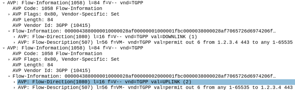
permit out 6 from 1.2.3.4 443 to any 1-65535
permit out 6 from any 1-65535 to 1.2.3.4 443
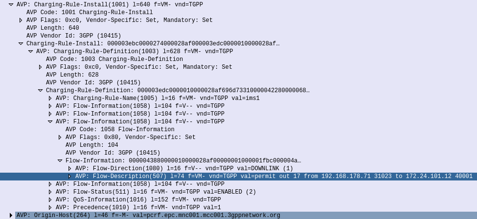
All this info gets put into the Flow-Information AVPs:
With the above, any traffic going to/from 1.23.4 on port 443, will match this rule (unless there’s another rule with a higher precedence value).
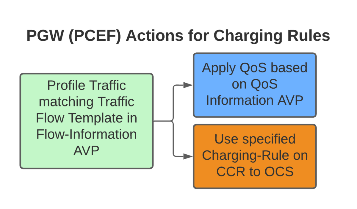
Charging Actions
So with our traffic profiled, the next question is what actions are we going to take, well there’s two, we’re going to provide unmetered access to the profiled traffic, and we’re going to use QCI 4 for the traffic (because you’ll need a guaranteed bit rate bearer to access!).
Charging-Group for Profiled Traffic
To allow for Zero Rating for traffic matching this rule, we’ll need to use a different Rating Group.
Let’s imagine our default rating group for data is 10000, then any normal traffic going to the OCS will use rating group 10000, and the OCS will apply the specific rates and policies based on that.
Rating Groups are defined in the OCS, and dictate what rates get applied to what Rating Groups.
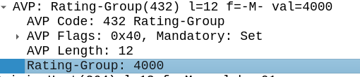
For us, our default rating group will be charged at the normal rates, but we can define a rating group value of 4000, and set the OCS to provide unlimited traffic to any Credit-Control-Requests that come in with Rating Group 4000.
This is how operators provide services like “Unlimited Facebook” for example, a Charging Rule matches the traffic to Facebook based on TFTs, and then the Rating Group is set differently to the default rating group, and the OCS just allows all traffic on that rating group, regardless of how much is consumed.
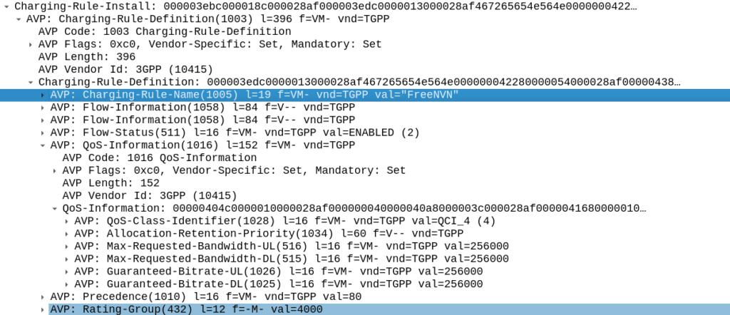
Inside our Charging-Rule-Definition, we populate the Rating-Group AVP to define what Rating Group we’re going to use.
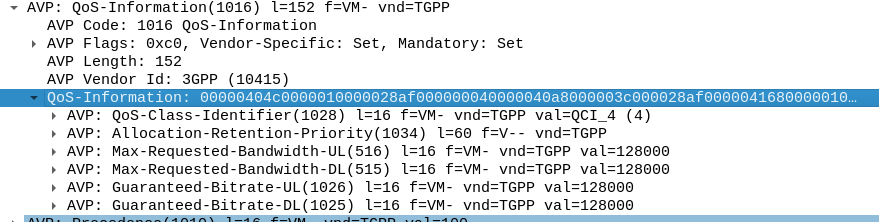
Setting QoS for Profiled Traffic
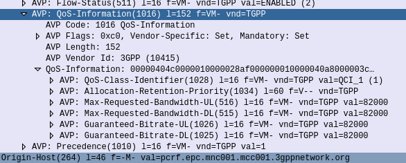
The QoS Description AVP defines which QoS parameters (QCI / ARP / Guaranteed & Maximum Bandwidth) should be applied to the traffic that matches the rules we just defined.
As mentioned at the start, we’ll use QCI 4 for this traffic, and allocate MBR/GBR values for this traffic.
Putting it Together – The Charging Rule
So with our TFTs defined to match the traffic, our Rating Group to charge the traffic and our QoS to apply to the traffic, we’re ready to put the whole thing together.
So here it is, our “Free NVN” rule:
I’ve attached a PCAP of the flow to this post.
In our next post we’ll talk about how the PGW handles the installation of this rule.
Next we’ll need to define our rt_pyform config, this is a super simple 3 line config file that specifies the path of what we’re doing:
DirectoryPath = "."        # Directory to search
ModuleName = "script"      # Name of python file. Note there is no .py extension
FunctionName = "transform" # Python function to call
The DirectoryPath directive specifies where we should search for the Python code, and ModuleName is the name of the Python script, lastly we have FunctionName which is the name of the Python function that does the rewriting.
Now let’s write our Python function for the transformation.
The Python function much have the correct number of parameters, must return a string, and must use the name specified in the config.
The following is an example of a function that prints out all the values it receives:
Note the order of the arguments and that return is of the same type as the AVP value (string).
We can expand upon this and add conditionals, let’s take a look at some more complex examples:
def transform(appId, flags, cmdCode, HBH_ID, E2E_ID, AVP_Code, vendorID, value):
    print('[PYTHON]')
    print(f'|-> appId: {appId}')
    print(f'|-> flags: {hex(flags)}')
    print(f'|-> cmdCode: {cmdCode}')
    print(f'|-> HBH_ID: {hex(HBH_ID)}')
    print(f'|-> E2E_ID: {hex(E2E_ID)}')
    print(f'|-> AVP_Code: {AVP_Code}')
    print(f'|-> vendorID: {vendorID}')
    print(f'|-> value: {value}')
    #IMSI Translation - if App ID = 16777251 and the AVP being evaluated is the Username
    if (int(appId) == 16777251) and int(AVP_Code) == 1:
        print("This is IMSI '" + str(value) + "' - Evaluating transformation")
        print("Original value: " + str(value))
        value = str(value[::-1]).zfill(15)
The above look at if the App ID is S6a, and the AVP being checked is AVP Code 1 (Username / IMSI ) and if so, reverses the username, so IMSI 1234567 becomes 7654321, the zfill is just to pad with leading 0s if required.
Now let’s do another one for a Realm Rewrite:
def transform(appId, flags, cmdCode, HBH_ID, E2E_ID, AVP_Code, vendorID, value):

    #Print Debug Info
    print('[PYTHON]')
    print(f'|-> appId: {appId}')
    print(f'|-> flags: {hex(flags)}')
    print(f'|-> cmdCode: {cmdCode}')
    print(f'|-> HBH_ID: {hex(HBH_ID)}')
    print(f'|-> E2E_ID: {hex(E2E_ID)}')
    print(f'|-> AVP_Code: {AVP_Code}')
    print(f'|-> vendorID: {vendorID}')
    print(f'|-> value: {value}')
    #Realm Translation
    if int(AVP_Code) == 283:
        print("This is Destination Realm '" + str(value) + "' - Evaluating transformation")
    if value == "epc.mnc001.mcc001.3gppnetwork.org":
        new_realm = "epc.mnc999.mcc999.3gppnetwork.org"
        print("translating from " + str(value) + " to " + str(new_realm))
        value = new_realm
    else:
        #If the Realm doesn't match the above conditions, then don't change anything
        print("No modification made to Realm as conditions not met")
    print("Updated Value: " + str(value))
In the above block if the Realm is set to epc.mnc001.mcc001.3gppnetwork.org it is rewritten to epc.mnc999.mcc999.3gppnetwork.org, hopefully you can get a handle on the sorts of transformations we can do with this – We can translate any string type AVPs, which allows for hostname, realm, IMSI, Sh-User-Data, Location-Info, etc, etc, to be rewritten.
NB-IoT introduces support for NIDD – Non-IP Data Delivery (NIDD) which is one of the cool features of NB-IoT that’s gaining more widespread adoption.
Let’s take a deep dive into NIDD.
The case against IP for IoT
In the over 40 years since IP was standardized, we’ve shoehorned many things onto IP, but IP was never designed or optimized for low power, low throughput applications.
For the battery life of an IoT device to be measured in years, it has to be very selective about what power hungry operations it does. Transmitting data over the air is one of the most power-intensive operations an IoT device can perform, so we need to do everything we can to limit how much data is sent, and how frequently.
Use Case – NB-IoT Tap
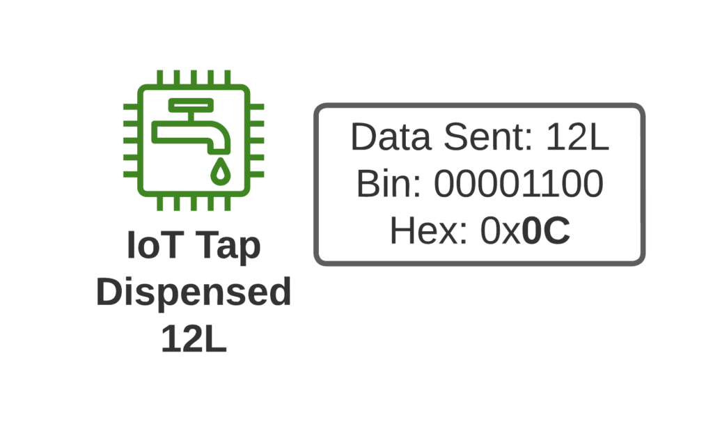
Let’s imagine we’re launching an IoT tap that transmits information about water used, as part of our revolutionary new “Water as a Service” model (WaaS) which removes the capex for residents building their own water treatment plant in their homes, and instead allows dynamic scaling of waterloads as they move to our new opex model.
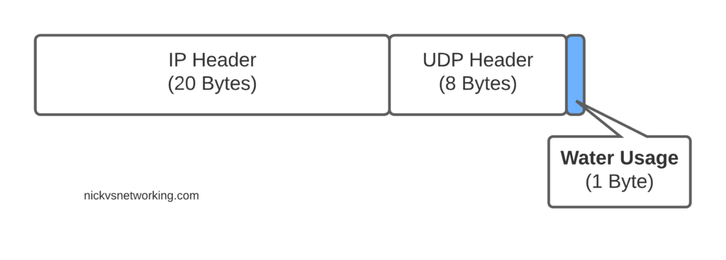
If I turn on the tap and use 12L of water, when I turn off the tap, our IoT tap encodes the usage onto a single byte and sends the usage information to our rain-cloud service provider.
So we’re not constantly changing the batteries in our taps, we need to send this one byte of data as efficiently as possible, so as to maximize the battery life.
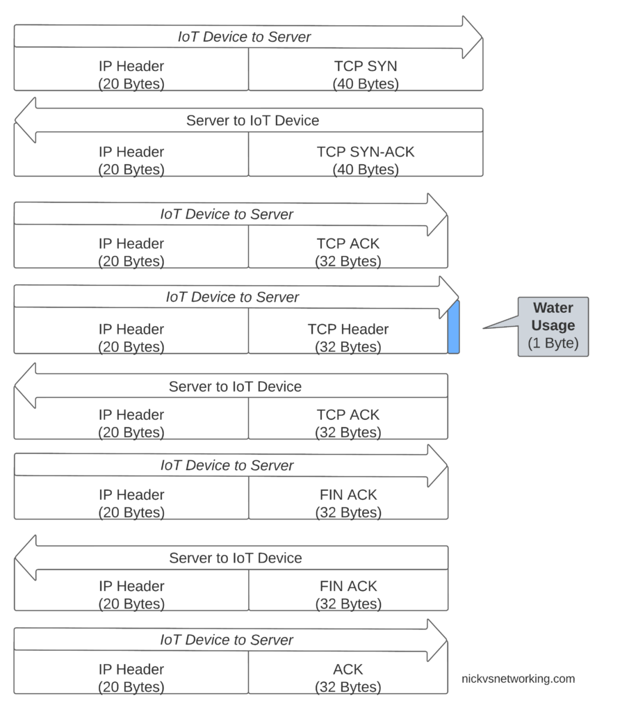
If we were to transport our data on TCP, well we’d need a 3 way handshake and several messages just to transmit the data we want to send.
Let’s see how our one byte of data would look if we transported it on TCP.
That sliver of blue in the diagram is our usage component, the rest is overhead used to get it there. Seems wasteful huh?
Sure, TCP isn’t great for this you say, you should use UDP! But even if we moved away from TCP to UDP, we’ve still got the IPv4 header and the UDP header wasting 28 bytes.
For efficiency’s sake (To keep our batteries lasting as long as possible) we want to send as few messages as possible, and where we do have to send messages, keep them very short, so IP is not a great fit here.
Enter NIDD – Non-IP Data Delivery.
Through NIDD we can just send the single hex byte, only be charged for the single hex byte, and only stay transmitting long enough to send this single byte of hex (Plus the NBIoT overheads / headers).
Compared to UDP transport, NIDD provides us a reduction of 28 bytes of overhead for each message, or a 96% reduction in message size, which translates to real power savings for our IoT device.
In summary – the more sending your device has to do, the more battery it consumes. So in a scenario where you’re trying to maximize power efficiency to keep your batter powered device running as long as possible, needing to transmit 28 bytes of wasted data to transport 1 byte of usable data, is a real waste.
Delivering the Payload
NIDD traffic is transported as raw hex data end to end, this means for our 1 byte of water usage data, the device would just send the hex value to be transferred and it’d pop out the other end.
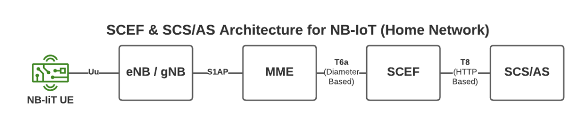
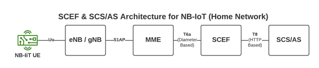
To support this we introduce a new network element called the SCEF –Service Capability Exposure Function.
From a developer’s perspective, the SCEF is the gateway to our IoT devices. Through the RESTful API on the SCEF (T8 API), we can send and receive raw hex data to any of our IoT devices.
When one of our Water-as-a-Service Taps sends usage data as a hex byte, it’s the software talking on the T8 API to the SCEF that receives this data.
Data of course needs to be addressed, so we know where it’s coming from / going to, and T8 handles this, as well as message reliability, etc, etc.
This is a telco blog, so we should probably cover the MME connection, the MME talks via Diameter to the SCEF. In our next post we’ll go into these signaling flows in more detail.
If you’re wondering what the status of Open Source SCEF implementations are, then you may have already guessed I’m working on one!
Hopefully by now you’ve got a bit of an idea of how NIDD works in NB-IoT, and in our next posts we’ll dig deeper into the flows and look at some PCAPs together.
Having a central pair of Diameter routing agents allows us to drastically simplify our network, but what if we want to perform some translations on AVPs?
For starters, what is an AVP transformation? Well it’s simply rewriting the value of an AVP as the Diameter Request/Response passes through the DRA. A request may come into the DRA with IMSI xxxxxx and leave with IMSI yyyyyy if a translation is applied.
So why would we want to do this?
Well, what if we purchased another operator who used Realm X, and we use Realm Y, and we want to link the two networks, then we’d need to rewrite Realm Y to Realm X, and Realm X to Realm Y when they communicate, AVP transformations allow for this.
If we’re an MVNO with hosted IMSIs from an MNO, but want to keep just the one IMSI in our HSS/OCS, we can translate from the MNO hosted IMSI to our internal IMSI, using AVP transformations.
If our OCS supports only one rating group, and we want to rewrite all rating groups to that one value, AVP transformations cover this too.
There are lots of uses for this, and if you’ve worked with a bit of signaling before you’ll know that quite often these sorts of use-cases come up.
So how do we do this with freeDiameter?
To handle this I developed a module for passing each AVP to a Python function, which can then apply any transformation to a text based value, using every tool available to you in Python.
In the next post I’ll introduce rt_pyform and how we can use it with Python to translate Diameter AVPs.
Way back in part 2 we discussed the basic routing logic a DRA handles, but what if we want to do something a bit outside of the box in terms of how we route?
For me, one of the most useful use cases for a DRA is to route traffic based on IMSI / Username. This means I can route all the traffic for MVNO X to MVNO X’s HSS, or for staging / test subs to the test HSS enviroment.
FreeDiameter has a bunch of built in logic that handles routing based on a weight, but we can override this, using the rt_default module.
In our last post we had this module commented out, but let’s uncomment it and start playing with it:
In the above code we’ve uncommented rt_default and rt_redirect.
You’ll notice that rt_default references a config file, so we’ll create a new file in our /etc/freeDiameter directory called rt_default.conf, and this is where the magic will happen.
A few points before we get started:
This overrides the default routing priorities, but in order for a peer to be selected, it has to be in an Open (active) state
The peer still has to have advertised support for the requested application in the CER/CEA dialog
The peers will still need to have all been defined in the freeDiameter.conf file in order to be selected
So with that in mind, and the 5 peers we have defined in our config above (assuming all are connected), let’s look at some rules we can setup using rt_default.
Intro to rt_default Rules
The rt_default.conf file contains a list of rules, each rule has a criteria that if matched, will result in the specified action being taken. The actions all revolve around how to route the traffic.
So what can these criteria match on? Here’s the options:
Item to Match
Code
Any
*
Origin-Host
oh=”STR/REG”
Origin-Realm
or=”STR/REG”
Destination-Host
dh=”STR/REG”
Destination-Realm
dr=”STR/REG”
User-Name
un=”STR/REG”
Session-Id
si=”STR/REG”
rt_default Matching Criteria
We can either match based on a string or a regex, for example, if we want to match anything where the Destination-Realm is “mnc001.mcc001.3gppnetwork.org” we’d use something like:
#Low score to HSS02
dr="mnc001.mcc001.3gppnetwork.org" : dh="hss02" += -70 ;
Now you’ll notice there is some stuff after this, let’s look at that.
We’re matching anything where the destination-host is set to hss02 (that’s the bit before the colon), but what’s the bit after that?
Well if we imagine that all our Diameter peers are up, when a message comes in with Destination-Realm “mnc001.mcc001.3gppnetwork.org”, looking for an HSS, then in our example setup, we have 4 HHS instances to choose from (assuming they’re all online).
In default Diameter routing, all of these peers are in the same realm, and as they’re all HSS instances, they all support the same applications – Our request could go to any of them.
But what we set in the above example is simply the following:
If the Destination-Realm is set to mnc001.mcc001.3gppnetwork.org, then set the priority for routing to hss02 to the lowest possible value.
So that leaves the 3 other Diameter peers with a higher score than HSS02, so HSS02 won’t be used.
Let’s steer this a little more,
Let’s specify that we want to use HSS01 to handle all the requests (if it’s available), we can do that by adding a rule like this:
#Low score to HSS02
dr="mnc001.mcc001.3gppnetwork.org" : dh="hss02" += -70 ;
#High score to HSS01
dr="mnc001.mcc001.3gppnetwork.org" : dh="hss01" += 100 ;
But what if we want to route to hss-lab if the IMSI matches a specific value, well we can do that too.
#Low score to HSS02
dr="mnc001.mcc001.3gppnetwork.org" : dh="hss02" += -70 ;
#High score to HSS01
dr="mnc001.mcc001.3gppnetwork.org" : dh="hss01" += 100 ;
#Route traffic for IMSI to Lab HSS
un="001019999999999999" : dh="hss-lab" += 200 ;
Now that we’ve set an entry with a higher score than hss01 that will be matched if the username (IMSI) equals 001019999999999999, the traffic will get routed to hss-lab.
But that’s a whole IMSI, what if we want to match only part of a field?
Well, we can use regex in the Criteria as well, so let’s look at using some Regex, let’s say for example all our MVNO SIMs start with 001012xxxxxxx, let’s setup a rule to match that, and route to the MVNO HSS with a higher priority than our normal HSS:
#Low score to HSS02
dr="mnc001.mcc001.3gppnetwork.org" : dh="hss02" += -70 ;
#High score to HSS01
dr="mnc001.mcc001.3gppnetwork.org" : dh="hss01" += 100 ;#Route traffic for IMSI to Lab HSS
un="001019999999999999" : dh="hss-lab" += 200 ;
#Route traffic where IMSI starts with 001012 to MVNO HSS
un=["^001012.*"] : dh="hss-mvno-x" += 200 ;
Let’s imagine that down the line we introduce HSS03 and HSS04, and we only want to use HSS01 if HSS03 and HSS04 are unavailable, and only to use HSS02 no other HSSes are available, and we want to split the traffic 50/50 across HSS03 and HSS04.
Firstly we’d need to add HSS03 and HSS04 to our FreeDiameter.conf file:
Then in our rt_default.conf we’d need to tweak our scores again:
#Low score to HSS02
dr="mnc001.mcc001.3gppnetwork.org" : dh="hss02" += 10 ;
#Medium score to HSS01
dr="mnc001.mcc001.3gppnetwork.org" : dh="hss01" += 20 ;
#Route traffic for IMSI to Lab HSS
un="001019999999999999" : dh="hss-lab" += 200 ;
#Route traffic where IMSI starts with 001012 to MVNO HSS
un=["^001012.*"] : dh="hss-mvno-x" += 200 ;
#High Score for HSS03 and HSS04dr="mnc001.mcc001.3gppnetwork.org" : dh="hss02" += 100 ;dr="mnc001.mcc001.3gppnetwork.org" : dh="hss04" += 100 ;
One quick tip to keep your logic a bit simpler, is that we can set a variety of different values based on keywords (listed below) rather than on a weight/score:
Behaviour
Name
Score
Do not deliver to peer (set lowest priority)
NO_DELIVERY
-70
The peer is a default route for all messages
DEFAULT
5
The peer is a default route for this realm
DEFAULT_REALM
10
REALM
15
Route to the specified Host with highest priority
FINALDEST
100
Rather than manually specifying the store you can use keywords like above to set the value
In our next post we’ll look at using FreeDiameter based DRA in roaming scenarios where we route messages across Diameter Realms.
FreeDiameter has been around for a while, and we’ve covered configuring the FreeDiameter components in Open5GS when it comes to the S6a interface, so you may have already come across FreeDiameter in the past, but been left a bit baffled as to how to get it to actually do something.
FreeDiameter is a FOSS implimentation of the Diameter protocol stack, and is predominantly used as a building point for developers to build Diameter applications on top of.
But for our scenario, we’ll just be using plain FreeDiameter.
So let’s get into it,
You’ll need FreeDiameter installed, and you’ll need a certificate for your FreeDiameter instance, more on that in this post.
Once that’s setup we’ll need to define some basics,
Inside freeDiameter.conf we’ll need to include the identity of our DRA, load the extensions and reference the certificate files:
What I typically refer to as Diameter interfaces / reference points, such as S6a, Sh, Sx, Sy, Gx, Gy, Zh, etc, etc, are also known as Applications.
Diameter Application Support
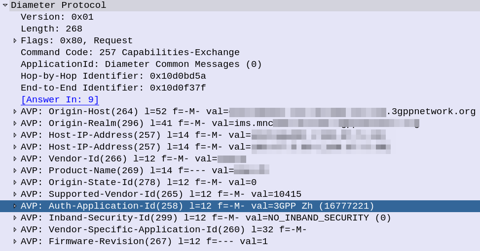
If you look inside the Capabilities Exchange Request / Answer dialog, what you’ll see is each side advertising the Applications (interfaces) that they support, each one being identified by an Application ID.
CER showing support for the 3GPP Zh Application-ID (Interface)
If two peers share a common Application-Id, then they can communicate using that Application / Interface.
For example, the above screenshot shows a peer with support for the Zh Interface (Spoiler alert, XCAP Gateway / BSF coming soon!). If two Diameter peers both have support for the Zh interface, then they can use that to send requests / responses to each other.
This is the basis of Diameter Routing.
Diameter Routing Tables
Like any router, our DRA needs to have logic to select which peer to route each message to.
For each Diameter connection to our DRA, it will build up a Diameter Routing table, with information on each peer, including the realm and applications it advertises support for.
Then, based on the logic defined in the DRA to select which Diameter peer to route each request to.
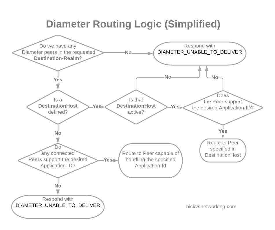
In its simplest form, Diameter routing is based on a few things:
Look at the DestinationRealm, and see if we have any peers at that realm
If we do then look at the DestinationHost, if that’s set, and the host is connected, and if it supports the specified Application-Id, then route it to that host
If no DestinationHost is specified, look at the peers we have available and find the one that supports the specified Application-Id, then route it to that host
Simplified Diameter Routing Table used by DRAs
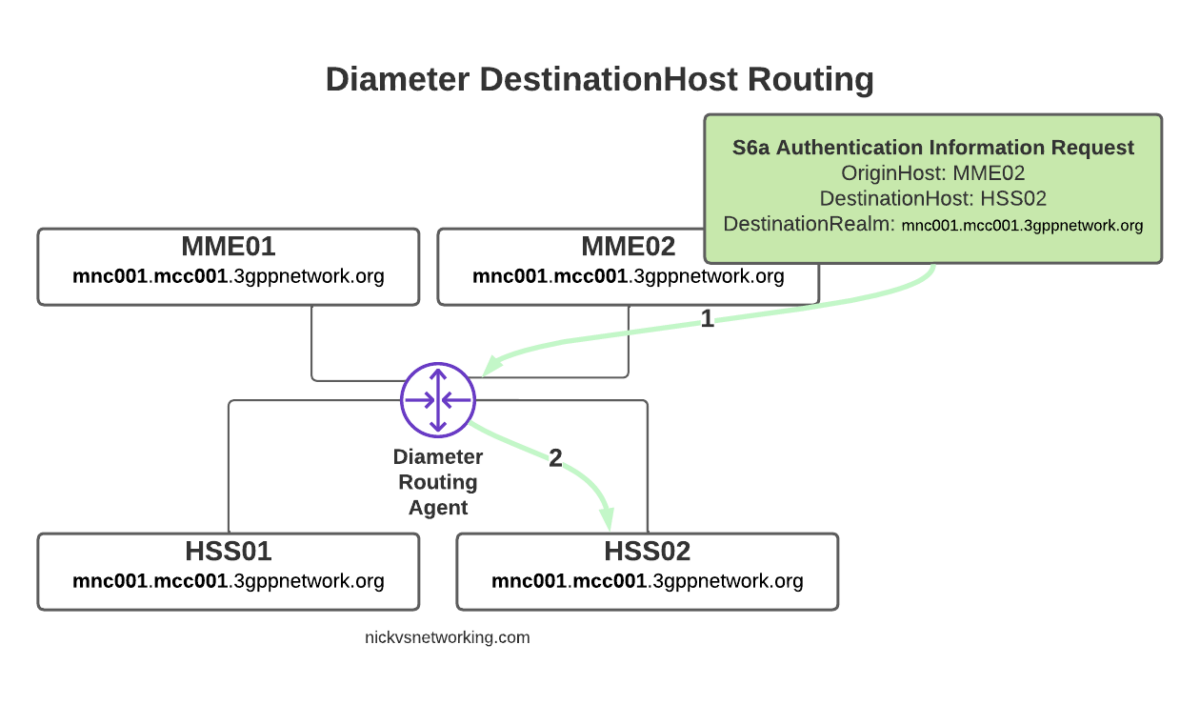
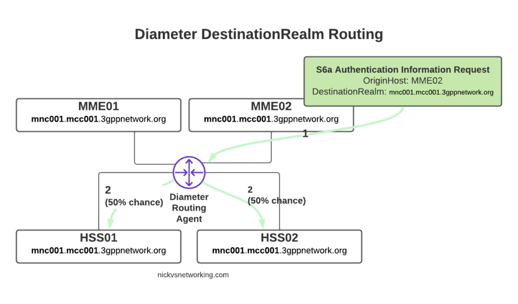
With this in mind, we can go back to looking at how our DRA may route a request from a connected MME towards an HSS.
Let’s look at some examples of this at play.
The request from MME02 is for DestinationRealm mnc001.mcc001.3gppnetwork.org, which our DRA knows it has 4 connected peers in (3 if we exclude the source of the request, as we don’t want to route it back to itself of course).
So we have 3 contenders still for who could get the request, but wait! We have a DestinationHost specified, so the DRA confirms the host is available, and that it supports the requested ApplicationId and routes it to HSS02.
So just because we are going through a DRA does not mean we can’t specific which destination host we need, just like we would if we had a direct link between each Diameter peer.
Conversely, if we sent another S6a request from MME01 but with no DestinationHost set, let’s see how that would look.
Again, the request is from MME02 is for DestinationRealm mnc001.mcc001.3gppnetwork.org, which our DRA knows it has 3 other peers it could route this to. But only two of those peers support the S6a Application, so the request would be split between the two peers evenly.
Clever Routing with DRAs
So with our DRA in place we can simplify the network, we don’t need to build peer links between every Diameter device to every other, but let’s look at some other ways DRAs can help us.
Load Control
We may want to always send requests to HSS01 and only use HSS02 if HSS01 is not available, we can do this with a DRA.
Or we may want to split load 75% on one HSS and 25% on the other.
Both are great use cases for a DRA.
Routing based on Username
We may want to route requests in the DRA based on other factors, such as the IMSI.
Our IMSIs may start with 001010001xxx, but if we introduced an MVNO with IMSIs starting with 001010002xxx, we’d need to know to route all traffic where the IMSI belongs to the home network to the home network HSS, and all the MVNO IMSI traffic to the MVNO’s HSS, and DRAs handle this.
Inter-Realm Routing
One of the main use cases you’ll see for DRAs is in Roaming scenarios.
For example, if we have a roaming agreement with a subscriber who’s IMSIs start with 90170, we can route all the traffic for their subs towards their HSS.
But wait, their Realm will be mnc901.mcc070.3gppnetwork.org, so in that scenario we’ll need to add a rule to route the request to a different realm.
DRAs handle this also.
In our next post we’ll start actually setting up a DRA with a default route table, and then look at some more advanced options for Diameter routing like we’ve just discussed.
One slight caveat, is that mutual support does not always mean what you may expect. For example an MME and an HSS both support S6a, which is identified by Auth-Application-Id 16777251 (Vendor ID 10415), but one is a client and one is a server. Keep this in mind!
Answer Question 1: Because they make things simpler and more flexible for your Diameter traffic. Answer Question 2: With free software of course!
All about DRAs
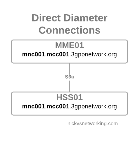
But let’s dive a little deeper. Let’s look at the connection between an MME and an HSS (the S6a interface).
Direct Diameter link between two Diameter Peers
We configure the Diameter peers on MME1 and HSS01 so they know about each other and how to communicate, the link comes up and presto, away we go.
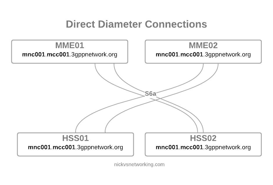
But we’re building networks here! N+1 redundancy and all that, so now we have two HSSes and two MMEs.
Direct Diameter link between 4 Diameter peers
Okay, bit messy, but that’s okay…
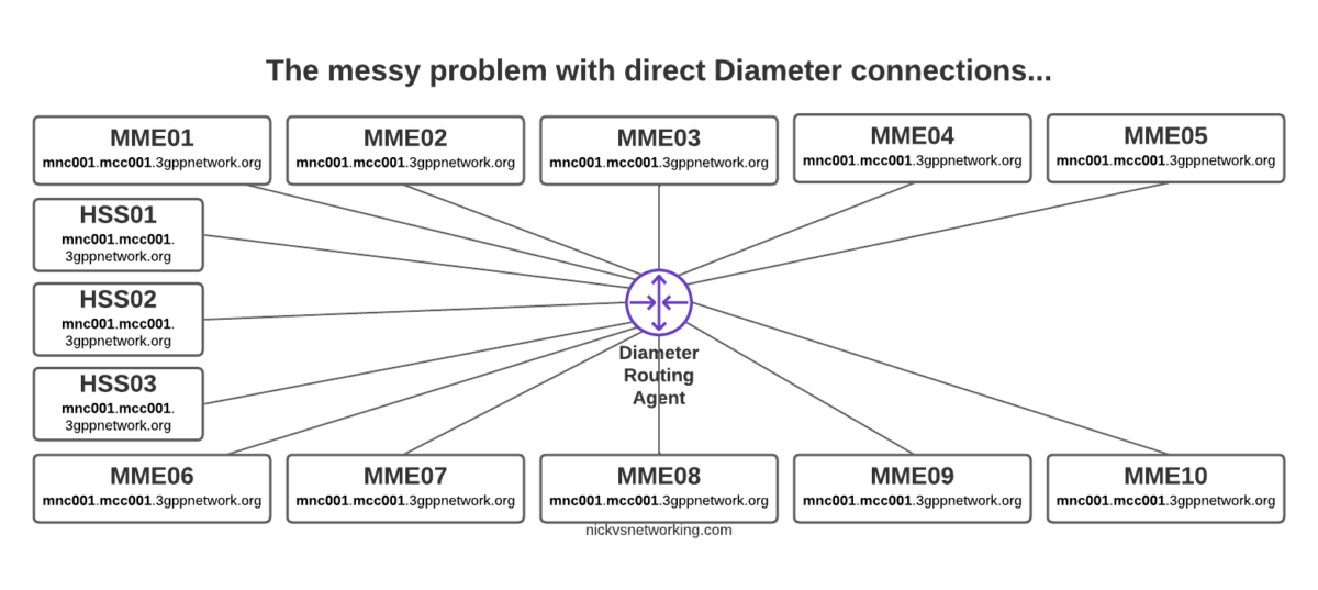
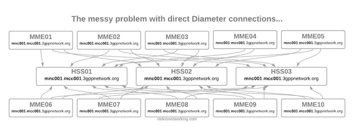
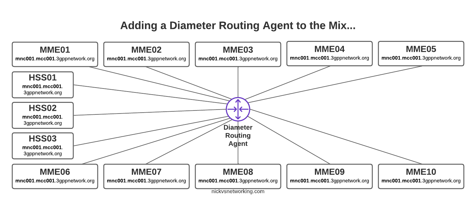
But then our network grows to 10 MMEs, and 3 HSSes and you can probably see where this is going, but let’s drive the point home.
Direct Diameter connections for a network with 10x MME and 3x HSS
Now imagine once you’ve set all this up you need to do some maintenance work on HSS03, so need to shut down the Diameter peer on 10 different MMEs in order to isolate it and deisolate it.
The problem here is pretty evident, all those links are messy, cumbersome and they just don’t scale.
If you’re someone with a bit of networking experience (and let’s face it, you’re here after all), then you’re probably thinking “What if we just had a central system to route all the Diameter messages?”
An Agent that could Route Diameter, a Diameter Routing Agent perhaps…
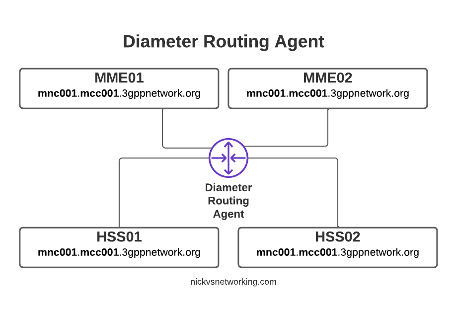
By introducing a DRA we build Diameter peer links between each of our Diameter devices (MME / HSS, etc) and the DRA, rather than directly between each peer.
With Diameter Routing Agent
Then from the DRA we can route Diameter requests and responses between them.
Let’s go back to our 10x MME and 3x HSS network and see how it looks with a DRA instead.
So much cleaner!
Not only does this look better, but it makes our life operating the network a whole lot easier.
Each MME sends their S6a traffic to the DRA, which finds a healthy HSS from the 3 and sends the requests to it, and relays the responses as well.
We can do clever load balancing now as well.
Plus if a peer goes down, the DRA detects the failure and just routes to one of the others.
If we were to introduce a new HSS, we wouldn’t need to configure anything on the MMEs, just add HSS04 to the DRA and it’ll start getting traffic.
Plus from an operations standpoint, now if we want to to take an HSS offline for maintenance, we just shut down the link on the HSS and all HSS traffic will get routed to the other two HSS instances.
In our next post we’ll talk about the Routing part of the DRA, how the decisions are made and all the nuances, and then in the following post we’ll actually build a DRA and start routing some traffic around!
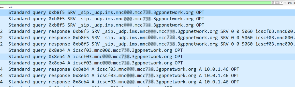
If you work with IMS or Packet Core, there’s a good chance you need DNS to work, and it doesn’t always.
When I run traces, I’ve always found I get swamped with DNS traffic, UE traffic, OS monitoring, updates, etc, all combine into a big firehose – while my Wireshark filters for finding EPC and IMS traffic is pretty good, my achilles heel has always been filtering the DNS traffic to just get the queries and responses I want out of it.
Well, today I made that a bit better.
By adding this to your Wireshark filter:
dns contains 33:67:70:70:6e:65:74:77:6f:72:6b:03:6f:72:67:00
You’ll only see DNS Queries and Responses for domains at the 3gppnetwork.org domain.
This makes my traces much easier to read, and hopefully will do the same for you!
Bonus, here’s my current Wireshark filter for working EPC/IMS:
(diameter and diameter.cmd.code != 280) or (sip and !(sip.Method == "OPTIONS") and !(sip.CSeq.method == "OPTIONS")) or (smpp and (smpp.command_id != 0x00000015 and smpp.command_id != 0x80000015)) or (mgcp and !(mgcp.req.verb == "AUEP") and !(mgcp.rsp.rspcode == 500)) or isup or sccp or rtpevent or s1ap or gtpv2 or pfcp or (dns contains 33:67:70:70:6e:65:74:77:6f:72:6b:03:6f:72:67:00)
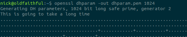
Even if you’re not using TLS in your FreeDiameter instance, you’ll still need a certificate in order to start the stack.
Luckily, creating a self-signed certificate is pretty simple,
Firstly we generate your a private key and public certificate for our required domain – in the below example I’m using dra01.epc.mnc001.mcc001.3gppnetwork.org, but you’ll need to replace that with the domain name of your freeDiameter instance.
If you’re using freeDiameter as part of another software stack (Such as Open5Gs) the below filenames will contain the config for that particular freeDiameter components of the stack:
So you have a VoIP service and you want to rate the calls to charge your customers?
You’re running a mobile network and you need to meter data used by subscribers?
Need to do least-cost routing?
You want to offer prepaid mobile services?
Want to integrate with Asterisk, Kamailio, FreeSWITCH, Radius, Diameter, Packet Core, IMS, you name it!
Well friends, step right up, because today, we’re talking CGrates!
So before we get started, this isn’t going to be a 5 minute tutorial, I’ve a feeling this may end up a big multipart series like some of the others I’ve done. There is a learning curve here, and we’ll climb it together – but it is a climb.
Installation
Let’s start with a Debian based OS, installation is a doddle:
We’re going to use Redis for the DataDB and MariaDB as the StorDB (More on these concepts later), you should know that other backend options are available, but for keeping things simple we’ll just use these two.
Next we’ll get the database and config setup,
cd /usr/share/cgrates/storage/mysql/
./setup_cgr_db.sh root CGRateS.org localhost
cgr-migrator -exec=*set_versions -stordb_passwd=CGRateS.org
Lastly we’ll clone the config files from the GitHub repo:
In its simplest form, rating is taking a service being provided and calculating the cost for it.
The start of this series will focus on voice calls (With SMS, MMS, Data to come), where the callingparty (The person making the call) pays, so let’s imagine calling a Mobile number (Starting with 614) costs $0.22 per minute.
To perform rating we need to determine the Destination, the Rate to be applied, and the time to charge for.
For our example earlier, a call to a mobile (Any number starting with 614) should be charged at $0.22 per minute. So a 1 minute call will cost $0.22 and a 2 minute long call will cost $0.44, and so on.
We’ll also charge calls to fixed numbers (Prefix 612, 613, 617 and 617) at a flat $0.20 regardless of how long the call goes for.
So let’s start putting this whole thing together.
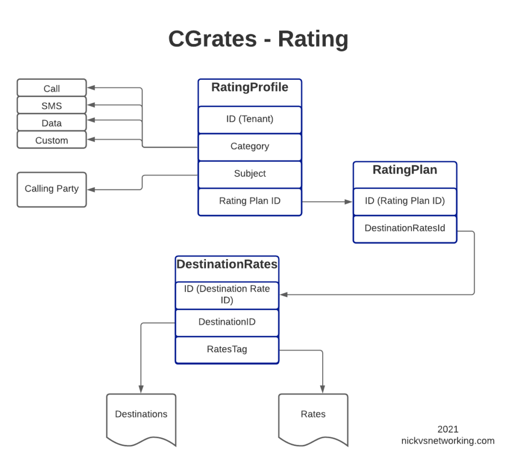
Introduction to RALs
RALs is the component in CGrates that takes care of Rating and Accounting Logic, and in this post, we’ll be looking at Rating.
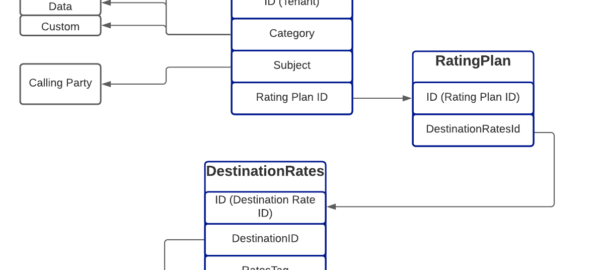
The rates have hierarchical structure, which we’ll go into throughout this post. I took my notepad doodle of how everything fits together and digitized it below:
Destinations
Destinations are fairly simple, we’ll set them up in our Destinations.csv file, and it will look something like this:
Each entry has an ID (referred to higher up as the Destination ID), and a prefix.
Also notice that some Prefixes share an ID, for example 612, 613, 617 & 618 are under the Destination ID named “DST_AUS_Fixed”, so a call to any of those prefixes would match DST_AUS_Fixed.
Rates
Rates define the price we charge for a service and are defined by our Rates.csv file.
This is nice and clean, a 1 second call costs $0.25, a 60 second call costs $0.25, and a 61 second call costs $0.50, and so on.
This is the standard billing mechanism for residential services, but it does not pro-rata the call – For example a 1 second call is the same cost as a 59 second call ($0.25), and only if you tick over to 61 seconds does it get charged again (Total of $0.50).
Per Second Billing
If you’re doing a high volume of calls, paying for a 3 second long call where someone’s voicemail answers the call and was hung up, may seem a bit steep to pay the same for that as you would pay for 59 seconds of talk time.
Instead Per Second Billing is more common for high volume customers or carrier-interconnects.
This means the rate still be set at $0.25 per minute, but calculated per second.
So the cost of 60 seconds of call is $0.25, but the cost of 30 second call (half a minute) should cost half of that, so a 30 second call would cost $0.125.
How often we asses the charging is defined by the RateIncrement parameter in the Rate Table.
We could achieve the same outcome another way, by setting the RateIncriment to 1 second, and the dividing the rate per minute by 60, we would get the same outcome, but would be more messy and harder to maintain, but you could think of this as $0.25 per minute, or $0.004166667 per second ($0.25/60 seconds).
Flat Rate Billing
Another option that’s commonly used is to charge a flat rate for the call, so when the call is answered, you’re charged that rate, regardless of the length of the call.
Regardless if the call is for 1 second or 10 hours, the charge is the same.
DestinationID – Refers to the DestinationID defined in the Destinations.csv file
RatesTag – Referes to the Rate ID we defined in Rates.csv
RoundingMethod – Defines if we round up or down
RoundingDecimals – Defines how many decimal places to consider before rounding
MaxCost – The maximum cost this can go up to
MaxCostStrategy – What to do if the Maximum Cost is reached – Either make the rest of the call Free or Disconnect the call
So for each entry we’ll define an ID, reference the Destination and the Rate to be applied, the other parts we’ll leave as boilerplate for now, and presto. We have linked our Destinations to Rates.
Rating Plans
We may want to offer different plans for different customers, with different rates.
DestinationRatesId (As defined in DestinationRates.csv)
TimingTag – References a time profile if used
Weight – Used to determine what precedence to use if multiple matches
So as you may imagine we need to link the DestinationRateIDs we just defined together into a Rating Plan, so that’s what I’ve done in the example above.
Rating Profiles
The last step in our chain is to link Customers / Subscribers to the profiles we’ve just defined.
How you allocate a customer to a particular Rating Plan is up to you, there’s numerous ways to approach it, but for this example we’re going to use one Rating Profile for all callers coming from the “cgrates.org” tenant:
Category is used to define the type of service we’re charging for, in this case it’s a call, but could also be an SMS, Data usage, or a custom definition.
Subject is typically the calling party, we could set this to be the Caller ID, but in this case I’ve used a wildcard “*any”
ActivationTime allows us to define a start time for the Rating Profile, for example if all our rates go up on the 1st of each month, we can update the Plans and add a new entry in the Rating Profile with the new Plans with the start time set
RatingPlanID sets the Rating Plan that is used as we defined in RatingPlans.csv
Loading the Rates into CGrates
At the start we’ll be dealing with CGrates through CSV files we import, this is just one way to interface with CGrates, there’s others we’ll cover in due time.
CGRates has a clever realtime architecture that we won’t go into in any great depth, but in order to load data in from a CSV file there’s a simple handy tool to run the process,
Obviously you’ll need to replace with the folder you cloned from GitHub.
Trying it Out
In order for CGrates to work with Kamailio, FreeSWITCH, Asterisk, Diameter, Radius, and a stack of custom options, for rating calls, it has to have common mechanisms for retrieving this data.
CGrates provides an API for rating calls, that’s used by these platforms, and there’s a tool we can use to emulate the signaling for call being charged, without needing to pickup the phone or integrate a platform into it.
The tenant will need to match those defined in the RatingProfiles.csv, the Subject is the Calling Party identity, in our case we’re using a wildcard match so it doesn’t matter really what it’s set to, the Destination is the destination of the call, AnswerTime is time of the call being answered (pretty self explanatory) and the usage defines how many seconds the call has progressed for.
The output is a JSON string, containing a stack of useful information for us, including the Cost of the call, but also the rates that go into the decision making process so we can see the logic that went into the price.
So have a play with setting up more Destinations, Rates, DestinationRates and RatingPlans, in these CSV files, and in our next post we’ll dig a little deeper… And throw away the CSVs all together!
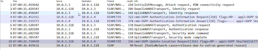
This post is one of a series of packet capture analysis challenges designed to test your ability to understand what is going on in a network from packet captures. Download the Packet Capture and see how many of the questions you can answer from the attached packet capture.
The answers are at the bottom of this page, along with how we got to the answers.
This challenge focuses on the Evolved Packet Core, specifically the S1 and Diameter interfaces.
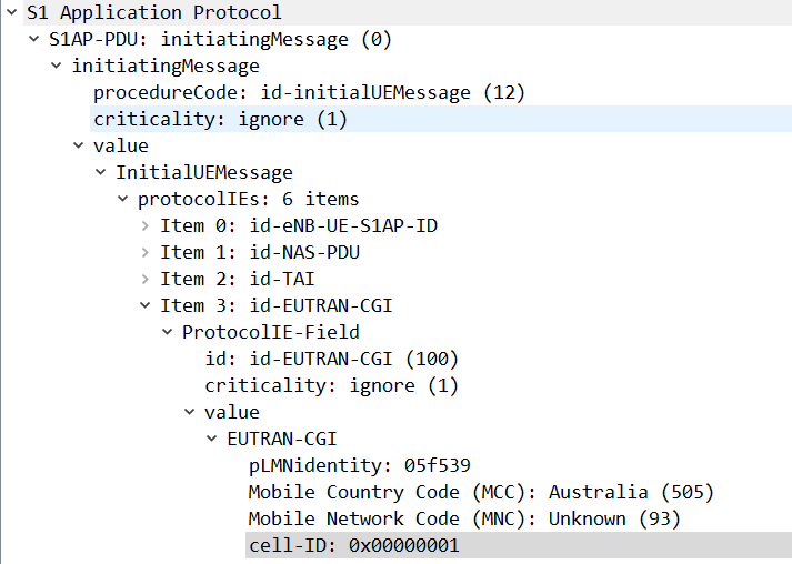
In Uplink messages from the eNodeB the EUTRAN-GCI field contains the Cell-ID of the eNodeB.
In this case the Cell-ID is 1.
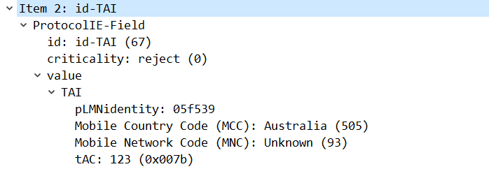
Answer: What is the Tracking Area?
The tracking area is 123.
This information is available in the TAI field in the Uplink S1 messages.
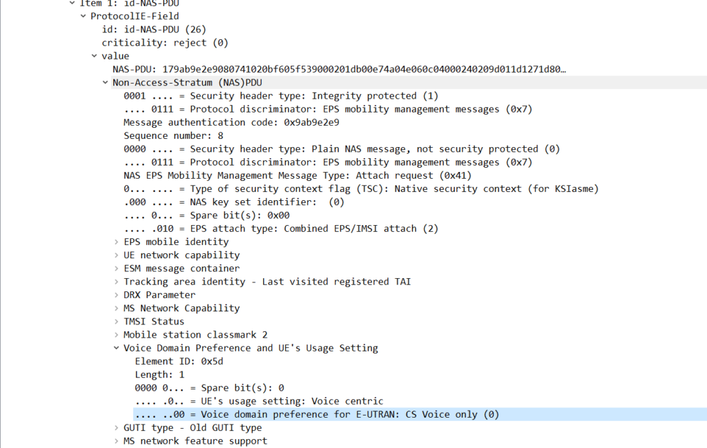
Answer: Does the device attaching to the network support VoLTE?
No, the device does not support VoLTE.
There are a few ways we can get to this answer, and VoLTE support in the phone does not mean VoLTE will be enabled, but we can see the Voice Domain preference is set to CS Voice Only, meaning GSM/UMTS for voice calling.
This is common on cheaper handsets that do not support VoLTE.
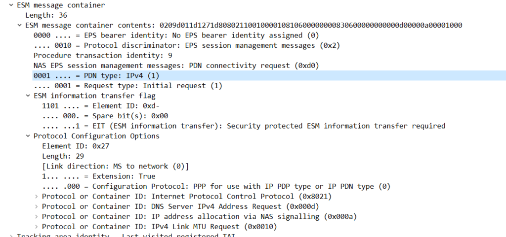
Answer: What type of IP is the subscriber requesting for this PDN session? (IPv4/IPv6/Both)?
The subscriber is requesting an IPv4 address only.
We can see this in the ESM Message Container for the PDN Connectivity Request, the PDN type is “IPv4”.
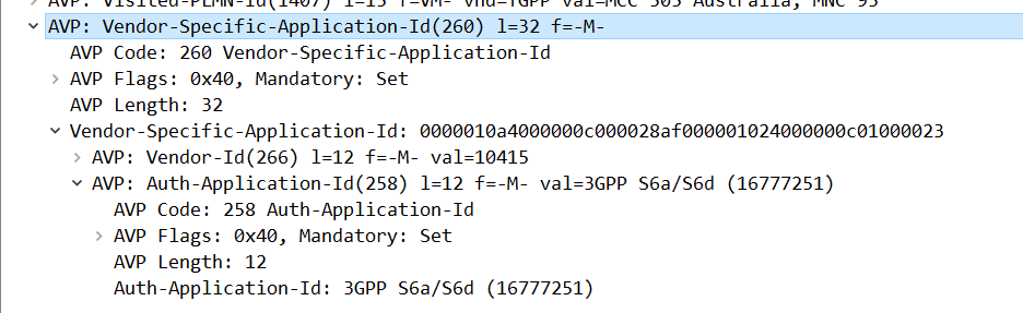
Answer: What is the Diameter Application ID for S6a?
Answer: 16777251
This is shown for the Vendor-Specific-Application-Id AVP on an S6a message.
Answer: What is the Crytpo RES returned by the HSS, and what is the RES returned by the SIM/UE?
The RES (Response) and X-RES (Expected Response) Both are “dba298fe58effb09“, they do match, which means this subscriber was authenticated successfully.
To support Dedicated Bearers we first have to have a way of profiling the traffic, to classify the traffic as being the type we want to provide the Dedicated Bearer for.
The first step involves a request from an Application Function (AF) to the PCRF via the Rx interface.
The most common type of AF would be a P-CSCF. When a VoLTE call gets setup the P-CSCF requests that a dedicated bearer be setup for the IP Address and Ports involved in the VoLTE call, to ensure users get the best possible call quality.
But Application Functions aren’t limited to just VoLTE – You could also embed an Application Function into the server for an online game to enable a dedicated bearer for users playing that game, or a sports streaming app that detects when a user starts streaming sports and creates a dedicated bearer for that user to send the traffic down.
The request to setup a dedicated bearer comes in the form of a Diameter request message from the AF, using the Rx reference point, typically from the P-CSCF to the PCRF in the network in an “AA-Request”.
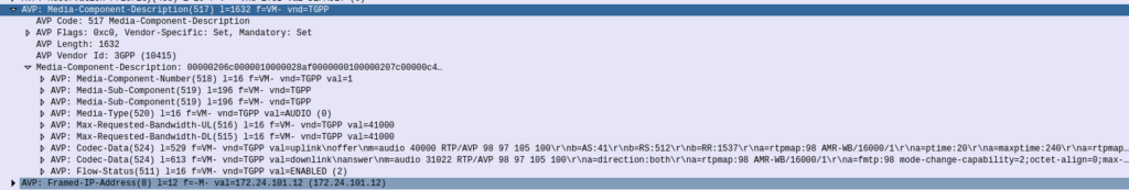
Of main interest in the AA-Request is the Media Component AVP, that contains all the details needed to identify the traffic flow.
Now our PCRF is in charge of policy, and know which P-GW is serving the required subscriber. So the PCRF takes this information and sends a Gx Re-Auth Request to the PCEF in the P-GW serving the subscriber, with a Charging Rule the PCEF in the P-GW needs to install, to profile and apply QoS to the bearer.
Charging Rule Definition’s Flow-Information AVPs showing the information needed to profile the traffic
The QoS Description AVP defines which QoS parameters (QCI / ARP / Guaranteed & Maximum Bandwidth) should be applied to the traffic that matches the rules we just defined.
QoS Information AVP showing requested QoS Parameters
The P-GW sends back a Gx Re-Auth Answer, and gets to work actually setting up these bearers.
With the rule installed on the PCEF, it’s time to get this new bearer set up on the UE / eNodeB.
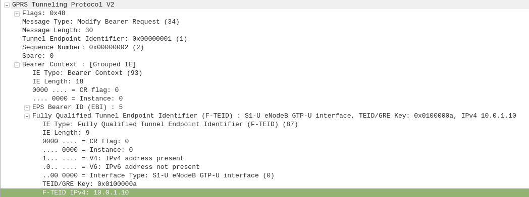
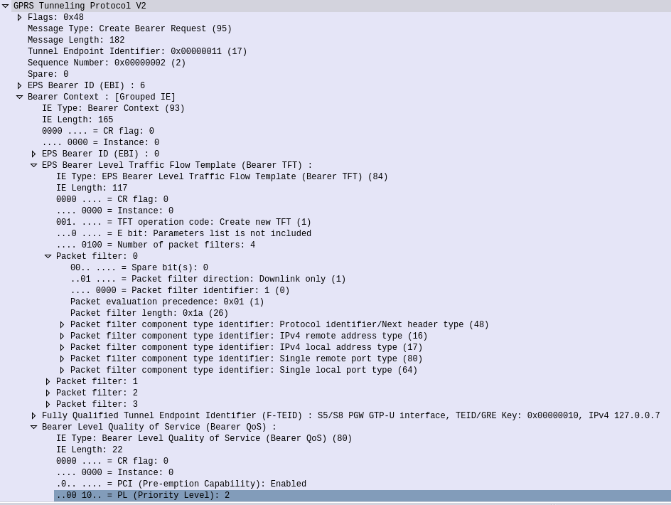
The P-GW sends a GTPv2 “Create Bearer Request” to the S-GW which forwards it onto the MME, to setup / define the Dedicated Bearer to be setup on the eNodeB.
GTPv2 “Create Bearer Request” sent by the P-Gw to the S-GW forwarded from the S-GW to the MME
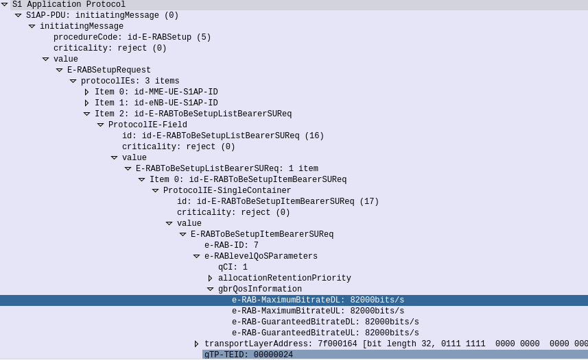
The MME translates this into an S1 “E-RAB Setup Request” which it sends to the eNodeB to setup,
S1 E-RAB Setup request showing the E-RAB to be setup
Assuming the eNodeB has the resources to setup this bearer, it provides the details to the UE and sets up the bearer, sending confirmation back to the MME in the S1 “E-RAB Setup Response” message, which the MME translates back into GTPv2 for a “Create Bearer Response”
All this effort to keep your VoLTE calls sounding great!
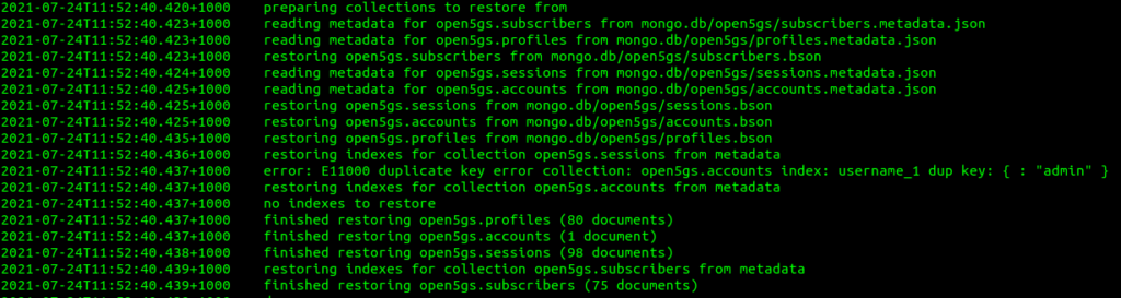
You may find you need to move your Open5GS deployments from one server to another, or split them between servers. This post covers the basics of migrating Open5GS config and data between servers by backing up and restoring it elsewhere.
The Database
Open5GS uses MongoDB as the database for the HSS and PCRF. This database contains all our SDM data, like our SIM Keys, Subscriber profiles, PCC Rules, etc.
Backup Database
To backup the MongoDB database run the below command (It doesn’t need sudo / root to run):
mongodump -o Open5Gs_"`date +"%d-%m-%Y"`"
You should get a directory called Open5Gs_todaysdate, the files in that directory are the output of the MongoDB database.
Restore Database
If you copy the backup we just took (the directory named Open5Gs_todaysdate) to the new server, you can restore the complete database by running:
mongorestore Open5Gs_todaysdate
This restores everything in the database, including profiles and user accounts for the WebUI,
You may instead just restore the Subscribers table, leaving the Profiles and Accounts unchanged with:
The database schema used by Open5GS changed earlier this year, meaning you cannot migrate directly from an old database to a new one without first making a few changes.
While reading through the 3GPP docs regarding Online Charging, there’s a concept that can be a tad confusing, and that’s the difference between Centralized and Non-Centralized Charging architectures.
The overall purpose of online charging is to answer that deceptively simple question of “does the user have enough credit for this action?”.
In order to answer that question, we need to perform rating and unit determination.
Rating
Rating is just converting connectivity credit units into monetary units.
If you go to the supermarket and they have boxes of Jaffa Cakes at $2.50 each, they have rated a box of Jaffa Cakes at $2.50.
1 Box of Jaffa Cakes rated at $2.50 per box
In a non-snack-cake context, such as 3GPP Online Charging, then we might be talking about data services, for example $1 per GB is a rate for data. Or for a voice calls a cost per minute to call a destination, such as is $0.20 per minute for a local call.
Rating is just working out the cost per connectivity unit (Data or Minutes) into a monetary cost, based on the tariff to be applied to that subscriber.
Unit Determination
The other key piece of information we need is the unit determination which is the calculation of the number of non-monetary units the OCS will offer prior to starting a service, or during a service.
This is done after rating so we can take the amount of credit available to the subscriber and calculate the number of non-monetary units to be offered.
Converting Hard-Currency into Soft-Snacks
In our rating example we rated a box of Jaffa Cakes at $2.50 per box. If I have $10 I can go to the shops and buy 4x boxes of Jaffa cakes at $2.50 per box. The cashier will perform unit determination and determine that at $2.50 per box and my $10, I can have 4 boxes of Jaffa cakes.
Again, steering away from the metaphor of the hungry author, Unit Determination in a 3GPP context could be determining how many minutes of talk time to be granted. Question: At $0.20 per minute to a destination, for a subscriber with a current credit of $20, how many minutes of talk time should they be granted? Answer: 100 minutes ($20 divided by $0.20 per minute is 100 minutes).
Or to put this in a data perspective, Question: Subscriber has $10 in Credit and data is rated at $1 per GB. How many GB of data should the subscriber be allowed to use? Answer: 10GB.
Putting this Together
So now we understand rating (working out the conversion of connectivity units into monetary units) and unit determination (determining the number of non-monetary units to be granted for a given resource), let’s look at the the Centralized and Decentralized Online Charging.
Centralized Rating
In Centralized Rating the CTF (Our P-GW or S-CSCF) only talk about non-monetary units. There’s no talk of money, just of the connectivity units used.
The CTFs don’t know the rating information, they have no idea how much 1GB of data costs to transfer in terms of $$$.
For the CTF in the P-GW/PCEF this means it talks to the OCS in terms of data units (data In/out), not money.
For the CTF in the S-CSCF this means it only ever talks to the OCS in voice units (minutes of talk time), not money.
This means our rates only need to exist in the OCS, not in the CTF in the other network elements. They just talk about units they need.
De-Centralized Rating
In De-Centralized Rating the CTF performs the unit conversion from money into connectivity units. This means the OCS and CTF talk about Money, with the CTF determining from that amount of money granted, what the subscriber can do with that money.
This means the CTF in the S-CSCF needs to have a rating table for all the destinations to determine the cost per minute for a call to a destination.
And the CTF in the P-GW/PCEF has to know the cost per octet transferred across the network for the subscriber.
In previous generations of mobile networks it may have been desirable to perform decentralized rating, as you can spread the load of calculating our the pricing, however today Centralized is the most common way to approach this, as ensuring the correct rates are in each network element is a headache.
Centralized Unit Determination
In Centralized Unit Determination the CTF tells the OCS the type of service in the Credit Control Request (Requested Service Units), and the OCS determines the number of non-monetary units of a certain service the subscriber can consume.
The CTF doesn’t request a value, just tells the OCS the service being requested and subscriber, and the OCS works out the values.
For example, the S-CSCF specifies in the Credit Control Request the destination the caller wishes to reach, and the OCS replies with the amount of talk time it will grant.
Or for a subscriber wishing to use data, the P-GW/PCEF sends a Credit Control Request specifying the service is data, and the OCS responds with how much data the subscriber is entitled to use.
De-Centralized Unit Determination
In De-Centralized Unit Determination, the CTF determines how many units are required to start the service, and requests these units from the OCS in the Credit Control Request.
For a data service,the CTF in the P-GW would determine how many data units it is requesting for a subscriber, and then request that many units from the OCS.
For a voice call a S-CSCF may request an initial call duration, of say 5 minutes, from the OCS. So it provides the information about the destination and the request for 300 seconds of talk time.
Session Charging with Unit Reservation (SCUR)
Arguably the most common online charging scenario is Session Charging with Unit Reservation (SCUR).
SCUR relies on reserving an amount of funds from the subscriber’s balance, so no other services can those funds and translating that into connectivity units (minutes of talk time or data in/out based on the Requested Session Unit) at the start of the session, and then subsequent requests to debit the reserved amount and reserve a new amount, until all the credit is used.
This uses centralized Unit Determination and centralized Rating.
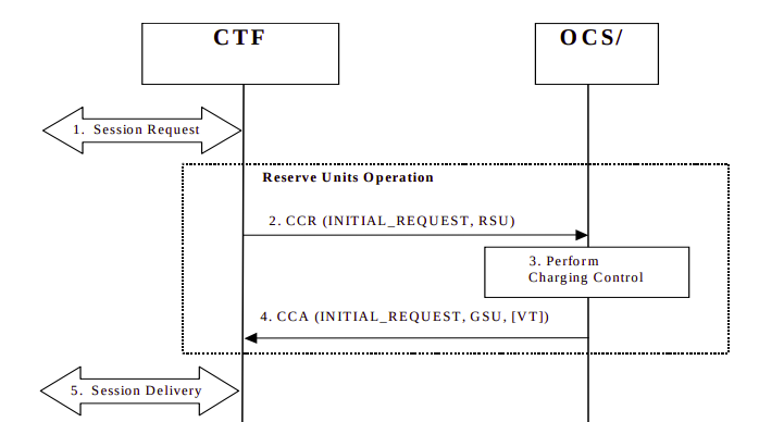
Let’s take a look at how this would look for the CTF in a P-GW/PCEF performing online charging for a subscriber wishing to use data:
Session Request: The subscriber has attached to the network and is requesting service.
The CTF built into the P-GW/PCEF sends a Credit Control Request: Initial Request (As this subscriber has just attached) to the OCS, with Requested Service Units (RSU) of data in/out to the OCS.
The OCS performs rating and unit determination, and according to it’s credit risk policies, and a whole lot of other factors, comes back with an amount of data the subscriber can use, and reserves the amount from the account. (It’s worth noting at this point that this is not necessarily all of the subscriber’s credit in the form of data, just an amount the OCS is willing to allocate. More data can be requested once this allocated data is used up.)
The OCS sends a Credit Control Answer back to our P-GW/PCEF. This contains the Granted Service Unit (GSU), in our case the GSU is data so defines much data up/down the user can transfer. It also may include a Validity Time (VT), which is the number of seconds the Credit Control Answer is valid for, after it’s expired another Credit Control Request must be sent by the CTF.
Our P-GW/PCEF processes this, starts measuring the data used by the subscriber for reporting later, and sets a timer for the Validity Time to send another CCR at that point. At this stage, our subscriber is able to start using data.
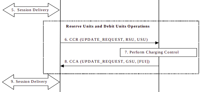
Some time later, either when all the data allocated in the Granted Service Units has been consumed, or when the Validity Time has expired, the CTF in the P-GW/PCEF sends another Credit Control Request:Update, and again includes the RSU (Requested Service Units) as data in/out, and also a USU (Used Service Units) specifying how much data the subscriber has used since the first Credit Control Answer.
The OCS receives this information. It compares the Used Session Units to the Granted Session Units from earlier, and with this is able to determine how much data the subscriber has actually used, and therefore how much credit that equates to, and debit that amount from the account. With this information the OCS can reserve more funds and allocate another GSU (Granted Session Unit) if the subscriber has the required balance. If the subscriber only has a small amount of credit left the FUI (Final Unit Indication AVP) is set to determine this is all the subscriber has left in credit, and if this is exhausted to end the session, rather than sending another Credit Control Request.
The Credit Control Answer with new GSU and the FUI is sent back to the P-GW/PCEF
The P-GW/PCEF allows the session to continue, again monitoring used traffic against the GSU (Granted Session Units).
Once the subscriber has used all the data in the Granted Session Units, and as the last CCA included the Final Unit Indicator, the CTF in the P-GW/PCEF knows it can’t just request more credit in the form of a CCR Update, so cuts of the subscribers’s session.
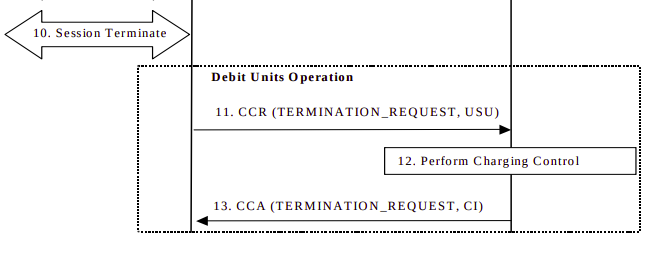
The P-GW/PCEF then sends a Credit Control Request: Termination Request with the final Used Service Units to the OCS.
The OCS debits the used service units from the subscriber’s balance, and refunds any unused credit reservation.
The OCS sends back a Credit Control Answer which may include the CI value for Credit Information, to denote the cost information which may be passed to the subscriber if required.
Early on as subscriber trunk dialing and automated time-based charging was introduced to phone networks, engineers were faced with a problem from Payphones.
Previously a call had been a fixed price, once the caller put in their coins, if they put in enough coins, they could dial and stay on the line as long as they wanted.
But as the length of calls began to be metered, it means if I put $3 of coins into the payphone, and make a call to a destination that costs $1 per minute, then I should only be allowed to have a 3 minute long phone call, and the call should be cutoff before the 4th minute, as I would have used all my available credit.
Conversely if I put $3 into the Payphone and only call a $1 per minute destination for 2 minutes, I should get $1 refunded at the end of my call.
We see the exact same problem with prepaid subscribers on IMS Networks, and it’s solved in much the same way.
In LTE/EPC Networks, Diameter is used for all our credit control, with all online charging based on the Ro interface. So let’s take a look at how this works and what goes on.
Generic 3GPP Online Charging Architecture
3GPP defines a generic 3GPP Online charging architecture, that’s used by IMS for Credit Control of prepaid subscribers, but also for prepaid metering of data usage, other volume based flows, as well as event-based charging like SMS and MMS.
Network functions that handle chargeable services (like the data transferred through a P-GW or calls through a S-CSCF) contain a Charging Trigger Function (CTF) (While reading the specifications, you may be left thinking that the Charging Trigger Function is a separate entity, but more often than not, the CTF is built into the network element as an interface).
The CTF is a Diameter application that generates requests to the Online Charging Function (OCF) to be granted resources for the session / call / data flow, the subscriber wants to use, prior to granting them the service.
So network elements that need to charge for services in realtime contain a Charging Trigger Function (CTF) which in turn talks to an Online Charging Function (OCF) which typically is part of an Online Charging System (AKA OCS).
For example when a subscriber turns on their phone and a GTP session is setup on the P-GW/PCEF, but before data is allowed to flow through it, a Diameter “Credit Control Request” is generated by the Charging Trigger Function (CTF) in the P-GW/PCEF, which is sent to our Online Charging Server (OCS).
The “Credit Control Answer” back from the OCS indicates the subscriber has the balance needed to use data services, and specifies how much data up and down the subscriber has been granted to use.
The P-GW/PCEF grants service to the subscriber for the specified amount of units, and the subscriber can start using data.
This is a simplified example – Decentralized vs Centralized Rating and Unit Determination enter into this, session reservation, etc.
The interface between our Charging Trigger Functions (CTF) and the Online Charging Functions (OCF), is the Ro interface, which is a Diameter based interface, and is common not just for online charging for data usage, IMS Credit Control, MMS, value added services, etc.
3GPP define a reference online-charging interface, the Ro interface, and all the application-specific interfaces, like the Gy for billing data usage, build on top of the Ro interface spec.
Basic Credit Control Request / Credit Control Answer Process
This example will look at a VoLTE call over IMS.
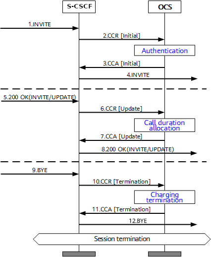
When a subscriber sends an INVITE, the Charging Trigger Function baked in our S-CSCF sends a Diameter “Credit Control Request” (CCR) to our Online Charging Function, with the type INITIAL, meaning this is the first CCR for this session.
The CCR contains the Service Information AVP. It’s this little AVP that is where the majority of the magic happens, as it defines what the service the subscriber is requesting. The main difference between the multitude of online charging interfaces in EPC networks, is just what the service the customer is requesting, and the specifics of that service.
For this example it’s a voice call, so this Service Information AVP contains a “IMS-Information” AVP. This AVP defines all the parameters for a IMS phone call to be online charged, for a voice call, this is the called-party, calling party, SDP (for differentiating between voice / video, etc.).
It’s the contents of this Service Information AVP the OCS uses to make decision on if service should be granted or not, and how many service units to be granted. (If Centralized Rating and Unit Determination is used, we’ll cover that in another post) The actual logic, relating to this decision is typically based on the the rating and tariffing, credit control profiles, etc, and is outside the scope of the interface, but in short, the OCS will make a yes/no decision about if the subscriber should be granted access to the particular service, and if yes, then how many minutes / Bytes / Events should be granted.
In the received Credit Control Answer is received back from our OCS, and the Granted-Service-Unit AVP is analysed by the S-CSCF. For a voice call, the service units will be time. This tells the S-CSCF how long the call can go on before the S-CSCF will need to send another Credit Control Request, for the purposes of this example we’ll imagine the returned value is 600 seconds / 10 minutes.
The S-CSCF will then grant service, the subscriber can start their voice call, and start the countdown of the time granted by the OCS.
As our chatty subscriber stays on their call, the S-CSCF approaches the limit of the Granted Service units from the OCS (Say 500 seconds used of the 600 seconds granted). Before this limit is reached the S-CSCF’s CTF function sends another Credit Control Request with the type UPDATE_REQUEST. This allows the OCS to analyse the remaining balance of the subscriber and policies to tell the S-CSCF how long the call can continue to proceed for in the form of granted service units returned in the Credit Control Answer, which for our example can be 300 seconds.
Eventually, and before the second lot of granted units runs out, our subscriber ends the call, for a total talk time of 700 seconds.
But wait, the subscriber been granted 600 seconds for our INITIAL request, and a further 300 seconds in our UPDATE_REQUEST, for a total of 900 seconds, but the subscriber only used 700 seconds?
The S-CSCF sends a final Credit Control Request, this time with type TERMINATION_REQUEST and lets the OCS know via the Used-Service-Unit AVP, how many units the subscriber actually used (700 seconds), meaning the OCS will refund the balance for the gap of 200 seconds the subscriber didn’t use.
If this were the interface for online charging of data, we’d have the PS-Information AVP, or for online charging of SMS we’d have the SMS-Information, and so on.
The architecture and framework for how the charging works doesn’t change between a voice call, data traffic or messaging, just the particulars for the type of service we need to bill, as defined in the Service Information AVP, and the OCS making a decision on that based on if the subscriber should be granted service, and if yes, how many units of whatever type.
While most users of Open5GS EPC will use NAT on the UPF / P-GW-U but you don’t have to.
While you can do NAT on the machine that hosts the PGW-U / UPF, you may find you want to do the NAT somewhere else in the network, like on a router, or something specifically for CG-NAT, or you may want to provide public addresses to your UEs, either way the default config assumes you want NAT, and in this post, we’ll cover setting up Open5GS EPC / 5GC without NAT on the P-GW-U / UPF.
Before we get started on that, let’s keep in mind what’s going to happen if we don’t have NAT in place,
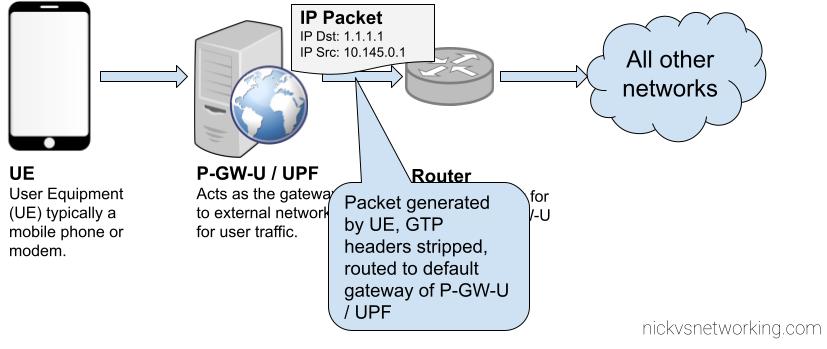
Traffic originating from users on our network (UEs / Subscribers) will have the from IP Address set to that of the UE IP Pool set on the SMF / P-GW-C, or statically in our HSS.
This will be the IP address that’s sent as the IP Source for all traffic from the UE if we don’t have NAT enabled in our Core, so all external networks will see that as the IP Address for our UEs / Subscribers.
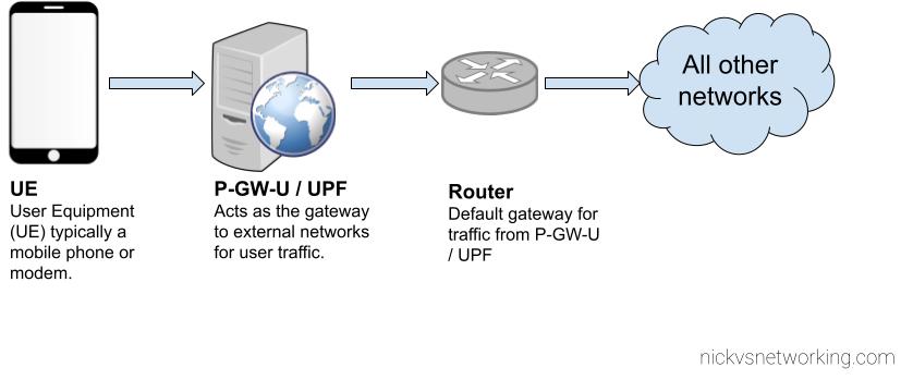
UE Generates packet
Core Network transports GTP encapsulated traffic to P-GW-U / UPF
UPF/P-GW-U routes the traffic to it’s default gateway
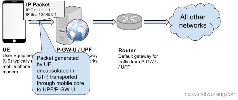
The above example shows the flow of a packet from UE with IP Address 10.145.0.1 sending something to 1.1.1.1.
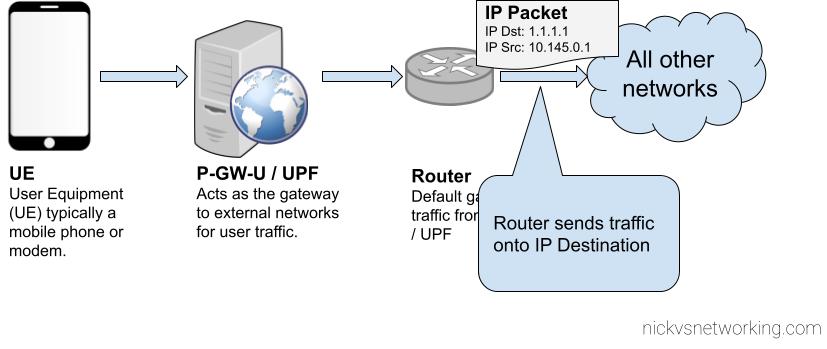
This is all well and good for traffic originating from our 4G/5G network, but what about traffic destined to our 4G/5G core?
Well, the traffic path is backwards. This means that our router, and external networks, need to know how to reach the subnet containing our UEs. This means we’ve got to add static routes to point to the IP Address of the UPF / P-GW-U, so it can encapsulate the traffic and get the GTP encapsulated traffic to the UE / Subscriber.
For our example packet destined for 1.1.1.1, as that is a globally routable IP (Not an internal IP) the router will need to perform NAT Translation, but for internal traffic within the network (On the router) the static route on the router should be able to route traffic to the UE Subnets to the UPF / P-GW-U’s IP Address, so it can encapsulate the traffic and get the GTP encapsulated traffic to the UE / Subscriber.
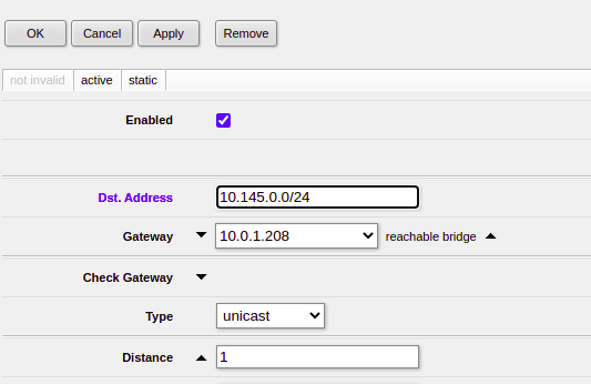
Setting up static routes on your router is going to be different on what you use, in my case I’m using a Mikrotik in my lab, so here’s a screenshot from that showing the static route point at my UPF/P-GW-U. I’ve got BGP setup to share routes around, so all the neighboring routers will also have this information about how to reach the subscriber.
Next up we’ve got to setup IPtables on the server itself running our UPF/P-GW-U, to route traffic addressed to the UE and encapsulate it.
sudo ip route add 10.145.0.0/24 dev ogstun
sudo echo 1 > /proc/sys/net/ipv4/ip_forward
sudo iptables -A FORWARD -i ogstun -o osgtun -s 10.145.0.0/24 -d 0.0.0.0/0 -j ACCEPT
And that’s it, now traffic coming from UEs on our UPF/P-GW will leave the NIC with their source address set to the UE Address, and so long as your router is happily configured with those static routes, you’ll be set.
If you want access to the Internet, it then just becomes a matter of configuring traffic from that subnet on the router to be NATed out your external interface on the router, rather than performing the NAT on the machine.
In an upcoming post we’ll look at doing this with OSPF and BGP, so you don’t need to statically assign routes in your routers.
While we’ve covered the Update Location Request / Response, where an MME is able to request subscriber data from the HSS, what about updating a subscriber’s profile when they’re already attached? If we’re just relying on the Update Location Request / Response dialog, the update to the subscriber’s profile would only happen when they re-attach.
We need a mechanism where the HSS can send the Request and the MME can send the response.
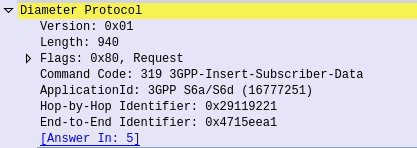
This is what the Insert Subscriber Data Request/Response is used for.
Let's imagine we want to allow a subscriber to access an additional APN, or change an AMBR values of an existing APN;

We'd send an Insert Subscriber Data Request from the HSS, to the MME, with the Subscription Data AVP populated with the additional APN the subscriber can now access.
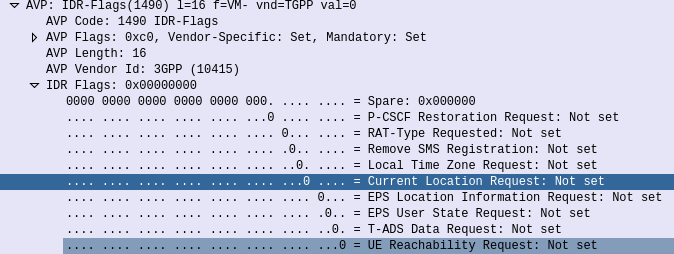
Beyond just updating the Subscription Data, the Insert Subscriber Data Request/Response has a few other funky uses.
Through it the HSS can request the EPS Location information of a Subscriber, down to the TAC / eNB ID serving that subscriber. It’s not the same thing as the GMLC interfaces used for locating subscribers, but will wake Idle UEs to get their current serving eNB, if the Current Location Request is set in the IDR Flags.
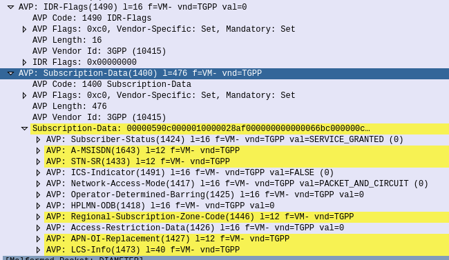
But the most common use for the Insert-Subscriber-Data request is to modify the Subscription Profile, contained in the Subscription-Data AVP,
If the All-APN-Configurations-Included-Indicator is set in the AVP info, then all the existing AVPs will be replaced, if it’s not then everything specified is just updated.
The Insert Subscriber Data Request/Response is a bit novel compared to other S6a requests, in this case it’s initiated by the HSS to the MME (Like the Cancel Location Request), and used to update an existing value.