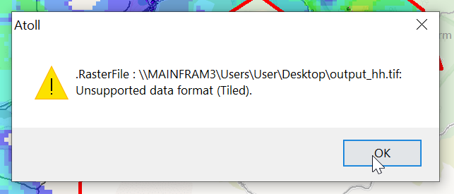
Looks like this is my 3rd (and hopefully final) post on the topic of loading Digital Elevation Models / Topographic data into Forsk Atoll, because this time, we’ve got global data, which allows us to Digital Elevation Models, at 30m resolution, for anywhere on the planet.
The Copernicus DEM is a Digital Surface Model (DSM) which represents the surface of the Earth including buildings, infrastructure and vegetation. This DSM is derived from an edited DSM named WorldDEM, where flattening of water bodies and consistent flow of rivers has been included. In addition, editing of shore- and coastlines, special features such as airports, and implausible terrain structures has also been applied.
The WorldDEM product is based on the radar satellite data acquired during the TanDEM-X Mission, which is funded by a Public Private Partnership between the German State, represented by the German Aerospace Centre (DLR) and Airbus Defence and Space. OpenTopography is providing access to the global GLO-30 Defence Gridded Elevation Data (DGED) 2023_1 version of the data hosted by ESA via the PRISM service. Details on the Copernicus DSM can be found on this ESA site.
This is a tool for a job, 30m resolution is not crazy high – LIDAR scans achieve sub 1m accuracy, but aren’t available everywhere, where as the COP30 dataset is global, meaning we can do RF design for anywhere on the planet.
So how do we get this into Atoll to do RF modeling?
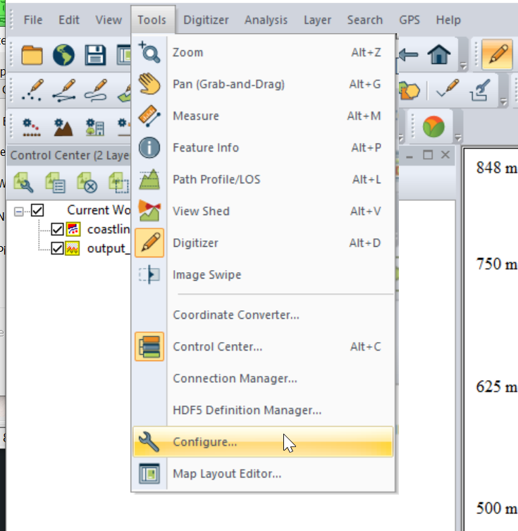
I had to re-project the data, so inside Global Mapper I had to go to Tools -> Configure.
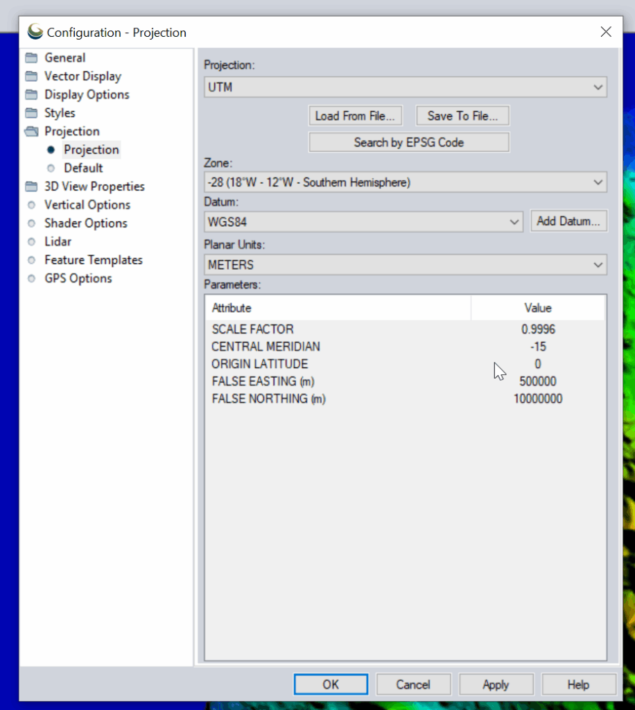
Then change the projection to UTM and use the UTM Zone Finder to find out what zone I needed.
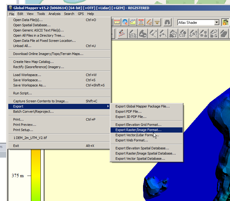
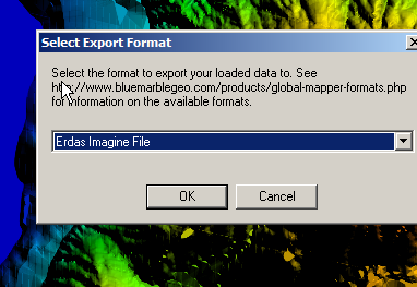
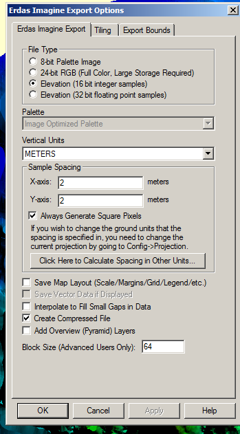
Then I exported the data as an Erdas Imagine file and was able to imported happily into Atoll, after setting the matching projection in Atoll (Which you generally do at the start of the project).
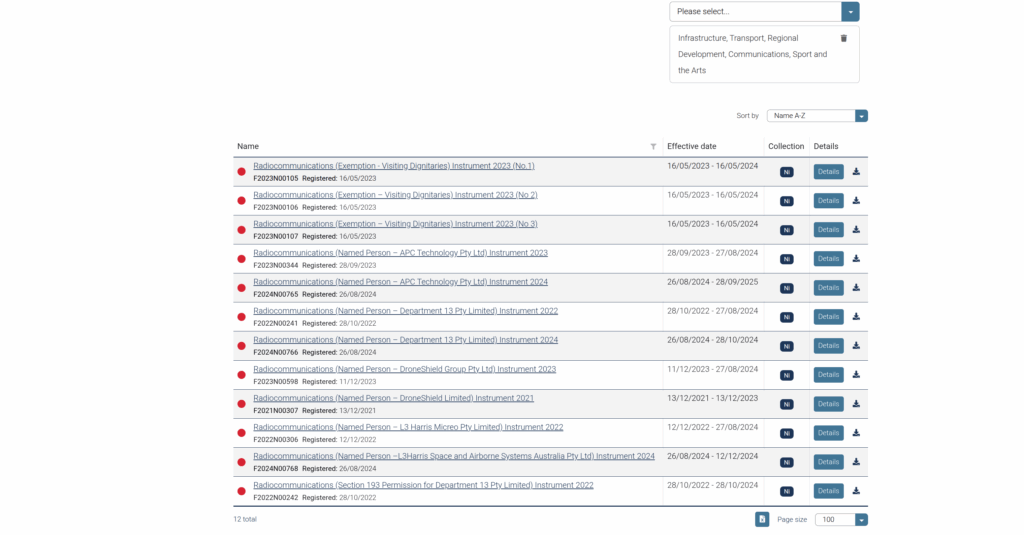
I got this email today from ACMA, the Australian communcations regulator who’s mailing list I subscribe to:
When I first started working, I’d often ride my motorbike to customer job sites with my cabling tools in a milk crate strapped on the back, but at no point did I combine customer cabling with riding the motorcycle – They seem like separate tasks.
So why does a motorbike race except certain people, equipment and cabling from the rules?
Will we see people on bikes traveling at great speed while crunching on Krone?
Leaning into the corners while working on lines?
Well, rather than doing my work I went down the rabbit hole to find out, and it started with ACMA gaving a handy link to the declaration in the email:
Section 54A Exemption – devices used for significant events says:
If you’re just operating your widgets for the purpose of a significant event, it’s cool, you don’t need to worry about complying with ACMA’s Low interference potential devices (LIPD) class license standards.
Section 54A Exemption – devices used for significant events (Some liberty taken)
So why would this exist?
Well, 5 days after the MotoGP wraps up on Philip Island it’s in Malaysia. I assume this loophole exists because there’s a lot of fancy telemetry stuff on the bikes, cameras, engine monitoring, lap time recording, and if MotoGP organizers had to get type-approval for everything and local cabling certification for everything, in every country the operate, when the race moves country to country each week, they’d never get approval for anything.
I did some research to see if this has been used before, and if so where, and came up short, this might be the first time this has been used:
What I did learn is if you’re a big enough wig (For example president of the US), you can get an exemption to the anti-jamming laws, which is used from time to time.
But as for the MotoGP being for their telemetry devices, this is just a guess, if anyone reading this knows definitively how this came to be, and where else this gets used, drop a comment – I’d be curious.
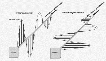
Let’s imagine the coin slot on a payphone – Coins can only enter the slot if they’re aligned with the slot.
If you tried to rotate the coin by 90 degrees, it wouldn’t fit it in the slot.
If the slot on the payphone went from up-to-down, our coin slot could be described as “vertically polarized”. Only coins in the vertically polarized orientation would fit.
Likewise, a payphone with the coin slot going side-to-side we could describe the coin slot as being “horizontally polarized”, meaning only coins that are horizontally polarized (on their side) would fit into the coin slot.
RF waves also have a polarization, like our coin slot.
A receiver wishing to receive into signals transmitted from a vertically-polarized antenna, will need to use a vertically-polarised antenna to pick up the signal.
Likewise a signal transmitted from a horizontally polarized antenna, would require a horizontally polarised antenna on the receiving side.
If there is a mismatch in polarization (for example RF waves transmitted from a horizontal polarized antenna but the receiver is using a vertically polarized antenna) the signal may still get through, but received signal strength would be severely degraded – in the order of 20dB, which is 1/100th of the power you’d get with the correct polarization.
You can think of polarization mismatches as like cutting up the coin to fit sideways through the coin slot – you’d get a sliver of the original coin that was cut up to fit. Much like you recieve a fraction of the original signal if your polarization doesn’t match on both ends.
Plagiarised diagram showing antenna polarization
Useless Information: In Australia country TV stations and metro TV stations sometimes transmitted different programming. To differentiate the signals on the receiver side, country TV transmitters used vertical polarisation, while metro transmitters used horizontal polarization. The use of different polarization orientation cuts down on interference in the border areas that sit in the footprint of the metro and country transmitters. This means as you drive through metro areas you’ll see all the yagi-antennas are horizontally oriented, while in country areas, they’re vertically oriented.
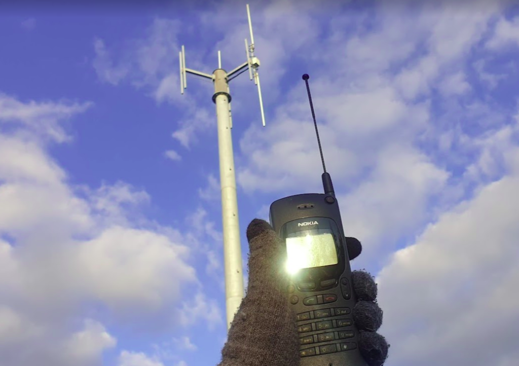
Vertical Polarization
Early mobile phone networks used Vertical Polarization.
This means they used an flagpole like antenna that is vertically oriented (Omnidirectional antenna) on the base-station sites.
Oldschool mobile phones also had a little pop out omnidirectional antenna, which when you held the phone to your ear, would orient the antenna vertically.
This matches with the antenna on the base station, and away we go. You still sometimes see vertical polarization in use on base-station sites in low density areas, or small cells.
Vertically polarized mobile phone antenna, which is oriented vertically, like on the base station behind it.
Increasing subscriber demand meant that operators needed more capacity in the network, but spectrum is expensive. As we just saw a mismatch in polarization can lead to a huge reduction in power, and maybe we can use that to our advantage…
Shannon-Hartley Theorem
But first, we need to do some maths…
Stick with me, this won’t be that hard to understand I promise.
There are two factors that influence the capacity of a network, the Bandwidth of the Channel and the Signal-to-Noise Ratio.
So let’s look at what each of these terms mean.
Bandwidth
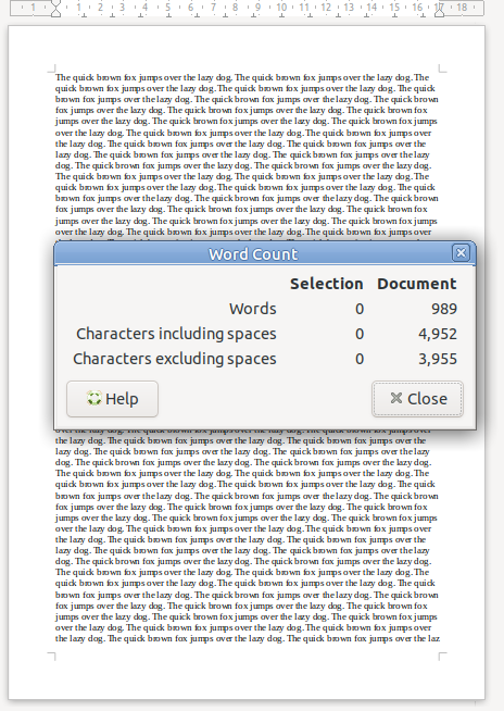
Bandwidth is the information carrying capacity. A one-page sheet of A4 at 12 point font, has a set bandwidth. There’s only so much text you can fit on one A4 sheet at that font size.
A4 Sheet, 12 point font, has 989 words.
We can increase the bandwidth two ways:
Option 1 to Increase Bandwidth: Get a larger transmission medium. Changing the size of the medium we’re working with, we can increase how much data we can transfer.
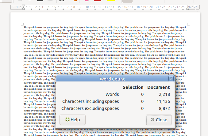
For this example we could get a bigger sheet of paper, for example an A3 sheet, or a billboard, will give us a lot more bandwidth (content carrying capability) than our sheet of A4.
Changing from an A4 sheet to an A3 sheet, increases the number of characters we can store on the page (Slightly more than doubling the bandwidth).
Option 2 to Increase Bandwidth: Use more efficient encoding As well as changing the size of the medium we are using, we can change how we store the data on the paper, for example, shrinking the font size to get more text in the same area, which also the bandwidth.
In communications networks this is also true: Bandwidth is determined by how much spectrum we have to work with (For example 10Mhz), and how we encode the data on that spectrum, ie morse-code, Binary-Phase-Shift-Keying or 16-QAM. Each of the different encoding schemes have different levels of bandwidth for the same amount of spectrum used, and we’ll cover those in more detail in the future.
So now we’ve covered increasing the bandwidth, now let’s talk about the other factor:
Signal-to-Noise Ratio
Signal-to-NoiseRatio (SNR) is the ratio of good signal, to the background noise.
On the train my headphones on block out most of the other sounds. In this scenario, the signal (the podcast I’m listening to on the headphones) is quite high, compared to the noise (unwanted sounds of other people on the train), so I have a good Signal-to-Noise ratio.
When we talk about the Signal-to-Noise Ratio, we’re talking about the ratio of the signal we want (podcast) to the noise (signal we don’t want).
When I’m on the train if 90% of what I hear is the podcast I’m listening to (the “signal”) and 10% is random background sounds (the “noise”) then my signal-to-noise-ratio is really good (high).
Capacity and SNR
Let’s continue with the listening to a podcast analogy.
The average human talks about 150 words per minute. So let’s imagine I’m listening to a podcast at 150 words per minute.
If I’m listening in an anechoic chamber, then I’ll be able to hear everything that’s being said, so my bandwidth will 150 words per minute. As there is no background noise, my capacity will also be 150 words per minute.
But if I leave an anechoic chamber (much as I love spending time in anechoic chambers), and go back on the train, I won’t hear the full 150 words per minute (bandwidth) due to the noise on the train drowning out some of the signal (podcast).
The Shannon-Hartley Theorem, states that the capacity is equal to the bandwidth multiplied by the signal to noise ratio.
So on the train hearing 90% of what’s said on the podcast, 10% drowned out, means my signal-to-noise ratio is 0.9 (pretty good).
So according to Shannon-Hartley Theorem the capacity of me listening to a podcast on the train (150 words per minute of bandwidth multiplied by 0.9 Signal-to-Noise Ratio) would give me 135 words per minute of capacity.
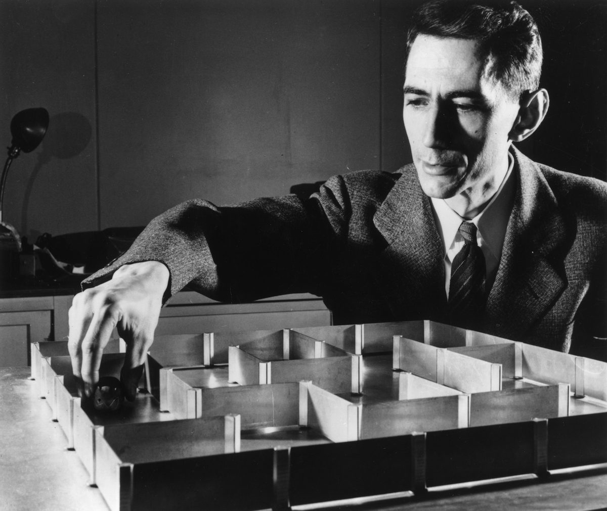
Claude Shannon, of 1/2 of the Shannon-Hartley Theorem, with an electromechanical mouse maze.
How this applies to RF Networks
In an RF context, our Bandwidth has a fixed information carrying capacity, for example on LTE, with a 5Mhz wide channel using 16QAM has 12.5Mbps of bandwidth available.
In a simple system, we have two levers we can pull to increase the bandwidth:
Increasing the size of the channel – If we went from a 5Mhz wide channel to a 20Mhz channel, this would give us 4x the available Bandwidth (Actually slightly more in LTE, but whatever)
Changing the encoding to cram more data on the same a size channel (From 16QAM to 64QAM would also give us 4x the available Bandwidth).
As we’ll see later in this post, there are some extra tricks (MIMO and Diversity) that we’ll look at later in this post, to increase the bandwidth of the system.
Our Signal-To-Noise (SNR) is constantly variable with a gazillion things that can influence the result. Some of the key factors that impact the SNR are the distance from the transmitter to the receiver and anything blocking the path between them (trees, buildings, mountains, etc), but there’s so many other factors that go into this. From atmospheric conditions, flat surfaces the signal can reflect off leading to multipath noise, other nearby transmitters, etc, can all influence our SNR.
Our capacity is equal to our Bandwidth multiplied by the Signal-to-Noise ratio.
Shannon-Hartley Theorem (ish)
As a goal we want capacity, and in an ideal world, our capacity would be equal to our bandwidth, but all that noise sneaks in and reduces our available capacity, based on the current SNR value.
So now we want to get more capacity out of the network, because everyone always wants to add capacity to networks.
One trick that we can use it to use multiple antennas with different polarization.
If our transmitter sends the same signal data out multiple antennas, with some clever processing on the transmitter and the receiver, we use this to maximize the received SNR. This is called Transmit Diversity and Receive Diversity and it’s a form of black magic.
The Transmitter uses feedback from the receiver to determine what the channel conditions are like, and then before transmitting the next block of data, compensates for the channel conditions experienced by the receiver, this increases the SNR and allows for higher MCS / encoding schemes, which in turns means higher throughput.
You’ll notice on most Antennas in the wild today you’ve got at least two ports for each frequency, which are + and -, which are the two polarizations.
Modern mobile networks use ±45° slant polarization (aka X Polarization), which works better in the orientations end users hold their phones in.
These two polarizations, each connected to a distinct transmit/receive path on the phone (UE) end and on the base station end, allows multiple data streams to be sent at the same time (spatial multiplexing, the foundation for MIMO) which enables higher throughput or can be configured enable redundancy in the transmission to better pick up weak signals (Diversity).
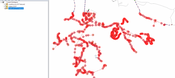
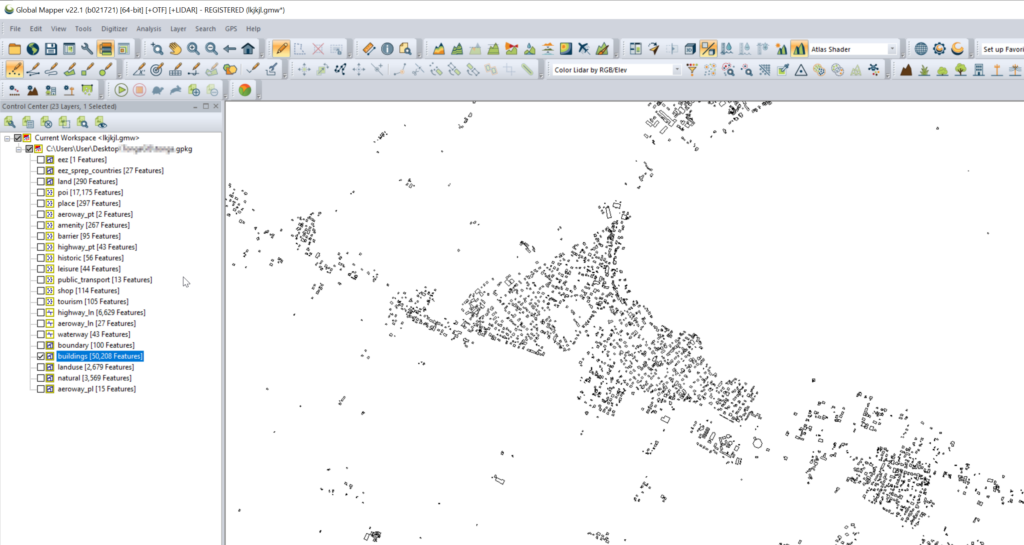
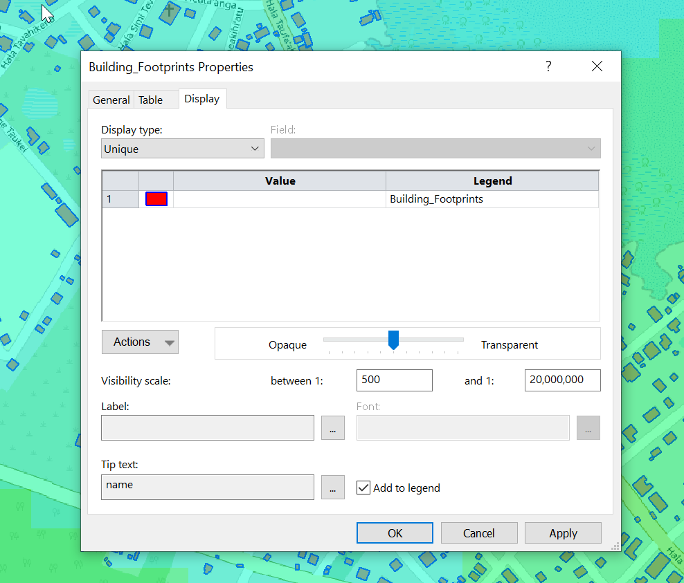
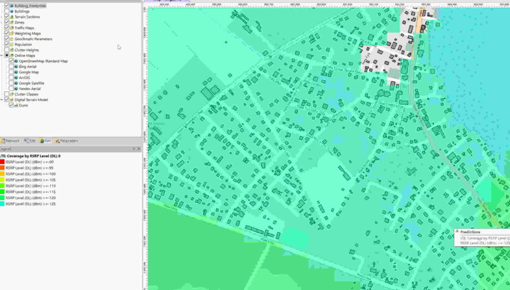
Having building footprints inside Atoll is super-duper valuable, this means you can calculate your percentage of homes / buildings covered, after all geographic coverage and population coverage are two very different things.
Once you’ve got the export, we’ll load the .gpkg file (or files) into GlobalMapper
Select one layer at a time that you want to export into Atoll. (This also works for roads, geographic boundaries, POIs, etc)
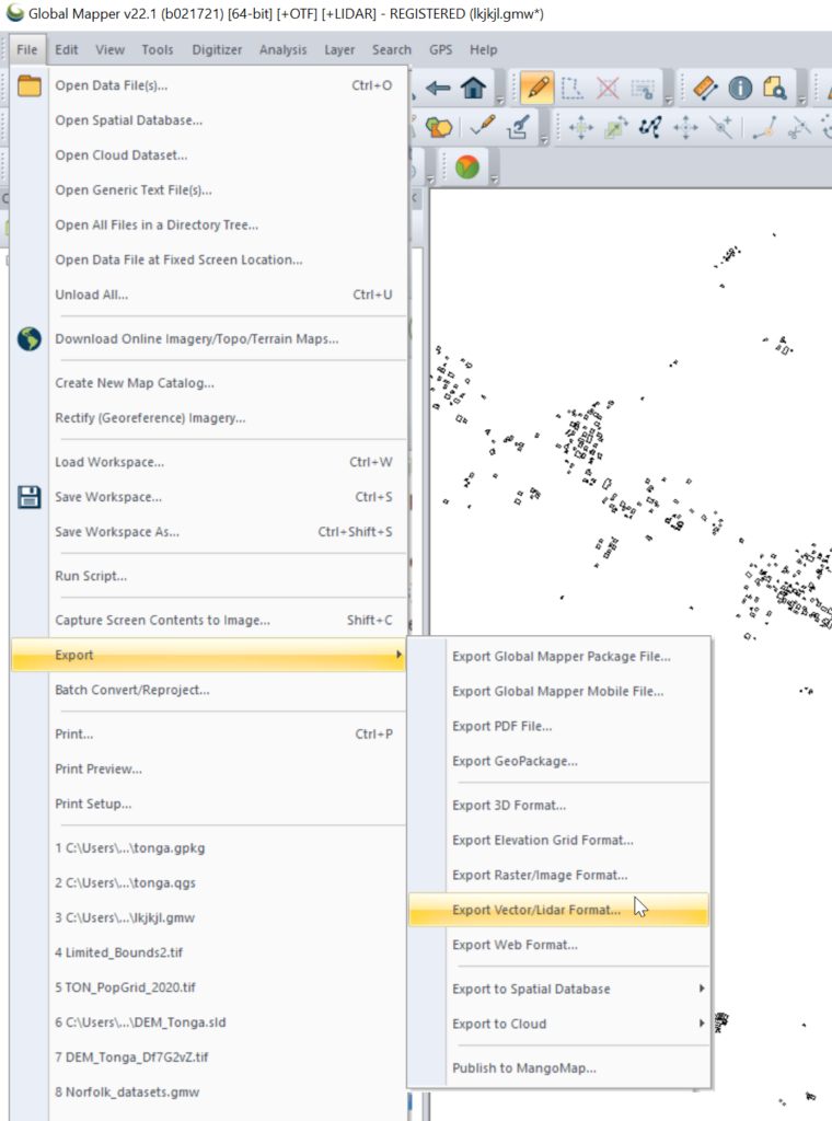
Export the selected layer from Export -> Export Vector / Lidar Format
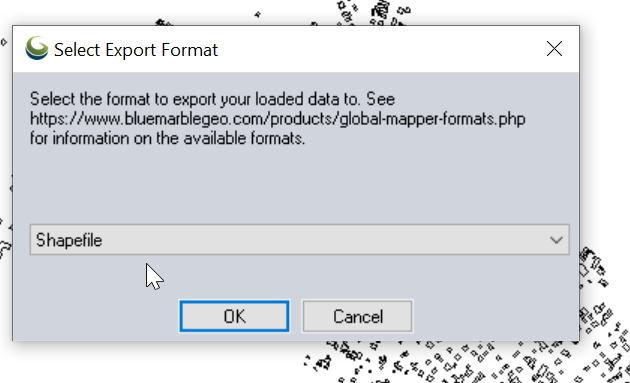
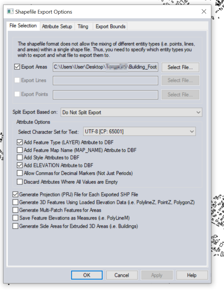
Set output type to “Shapefile”
Set output filename in “Export Areas” (This will be the output file). If you want to limit the export to a given area you can do that in Export Bounds.
Now we can import this data into Atoll.
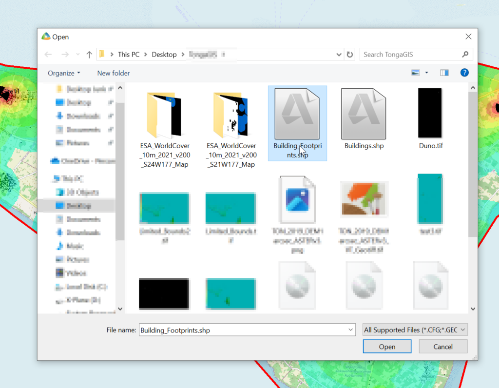
File -> Import
Select the exported Shapefile we just created.
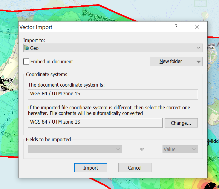
Set the projection and import
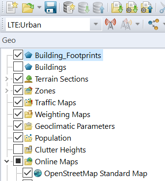
Bingo now we’ve got our building footprints,
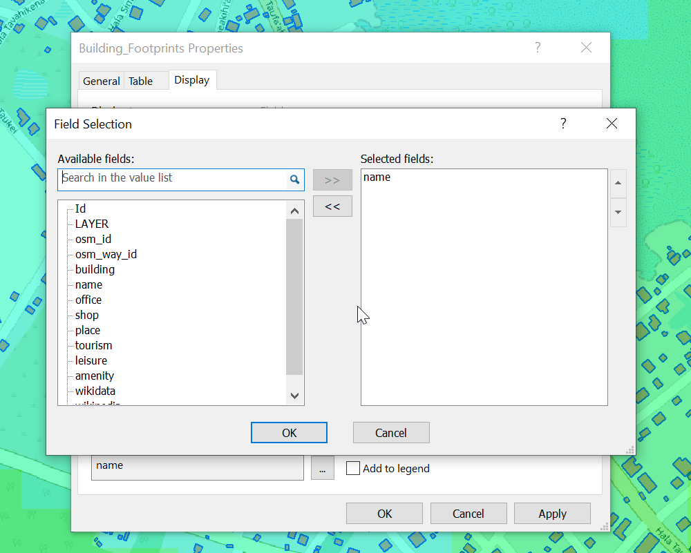
We can change the style of the layer and the labels as needed.
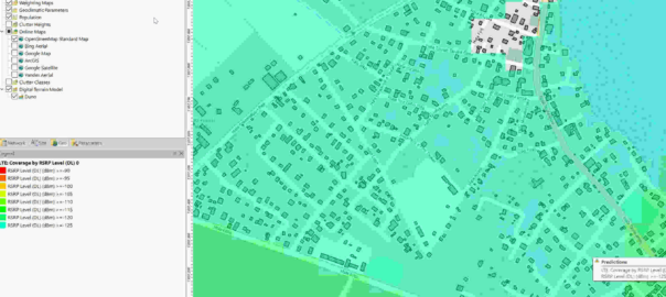
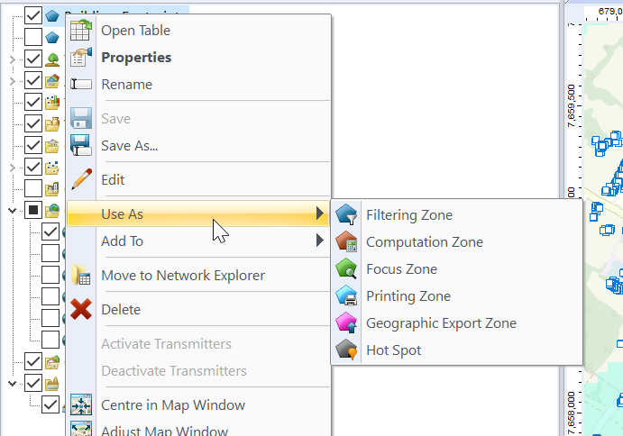
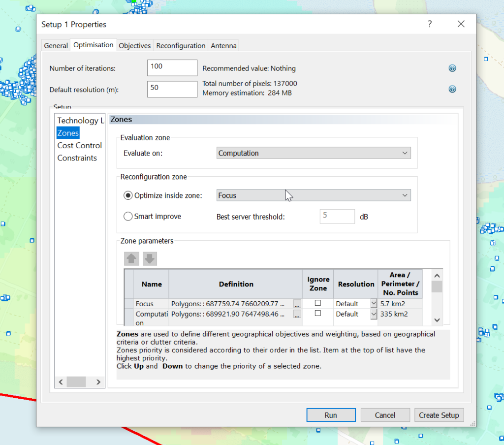
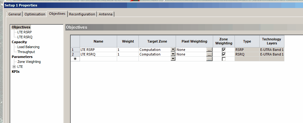
Now we can use the buildings as the Focus Zone / Compute Zone and then run reports and predictions based on those areas.
For example I can run Automatic Cell Planning with the building layers as the Focus zones, to optimize azimuths, tilts and powers to provide coverage to where people live, not just vacant land.
Clutter data describes real world things on the planet’s surface that attenuate signals, for example trees, shrubs, buildings, bodies of water, etc, etc. There’s also different types of trees, some types of trees attenuate signals more than others, different types of buildings are the same.
Getting clutter data used to be crazy expensive, and done on a per country or even per region basis, until the European Space Agency dropped a global dataset free of charge for anyone to use, that covered the entire planet in a single source of data.
So we can use this inside Forsk Atoll for making our predictions.
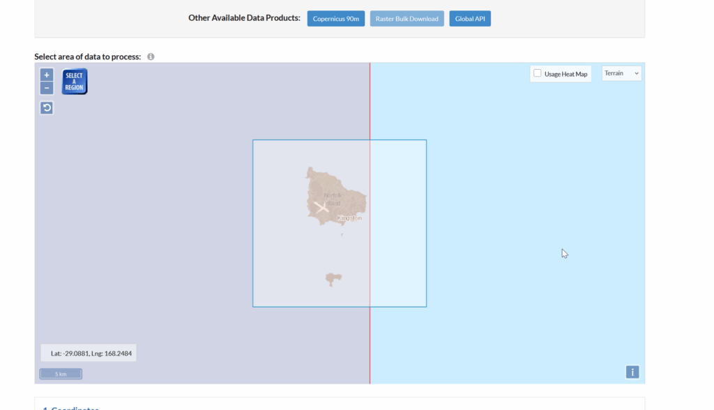
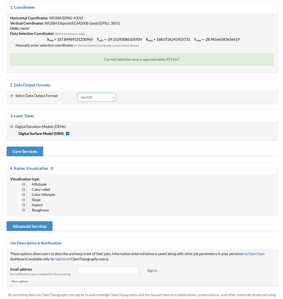
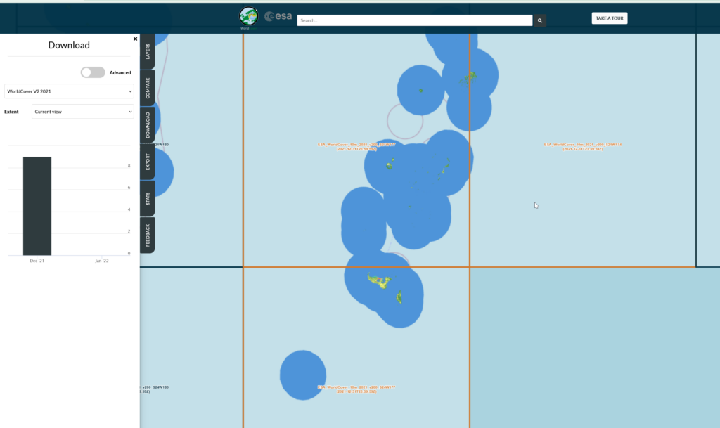
First things first we’ll need to create an account with the ESA (This is not where they take astronaut applications unfortunately, it just gives you access to the datasets).
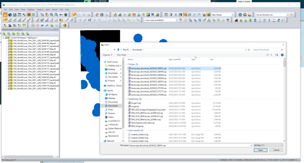
Then you can select the areas (tiles) you want to download after clicking the “Download” tab on the right.
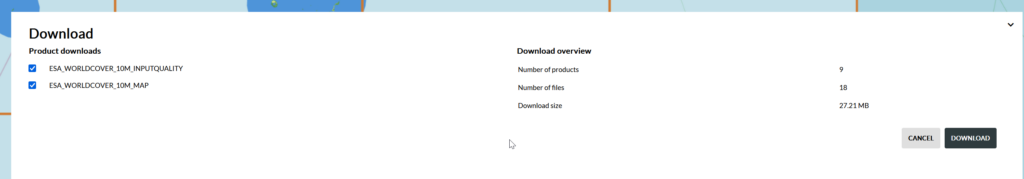
We get a confirmation of the tiles we’re download and we’ll get a ZIP file containing the data.
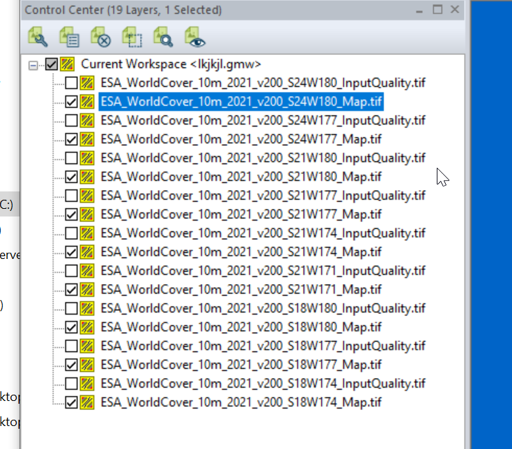
We can load the whole ZIP file (Without needing to extract anything) into GlobalMapper which loads all the layers.
I found the _Map.tif files the highest resolution, so I’m only exporting these.
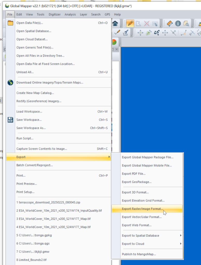
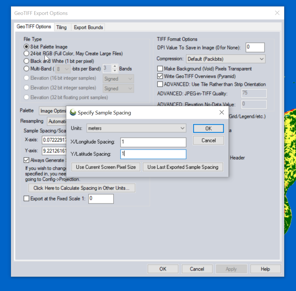
Then we need to export the data to GeoTiff for use in Atoll (The specific GeoTiff format ESA produces them in is not compatible with Atoll hence the need to convert), so we export the layers as Raster / Image format.
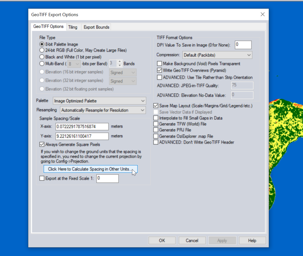
Atoll requires square pixels, and we need them in meters, so we select “Calculate Spacing in Other Units”.
Then set the spacing to meters (I use 1m to match everything else, but the data is actually only 10m accurate, so you could set this to 10m).
You probably want to set the Export Bounds to just the areas you’re interested in, otherwise the data gets really big, really quickly and takes forever to crunch.
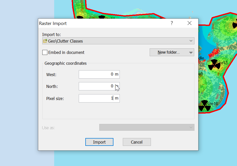
Now for the fancy part, we need to import it into Atoll.
When we import the data we import it as Raster data (Clutter Classes) with a pixel size of 1m.
Alas when we exported the data we’ve lost the positioning information, so while we’ve got the clutter data, it’s just there somewhere on the planet, which with the planet being the size it is, is probably not where you need it.
So I cheat, I start put putting the West and North values to match the values from a Cell Site I’ve already got on the map (I put one in the top left and bottom right corners of the map) and use that as the initial value.
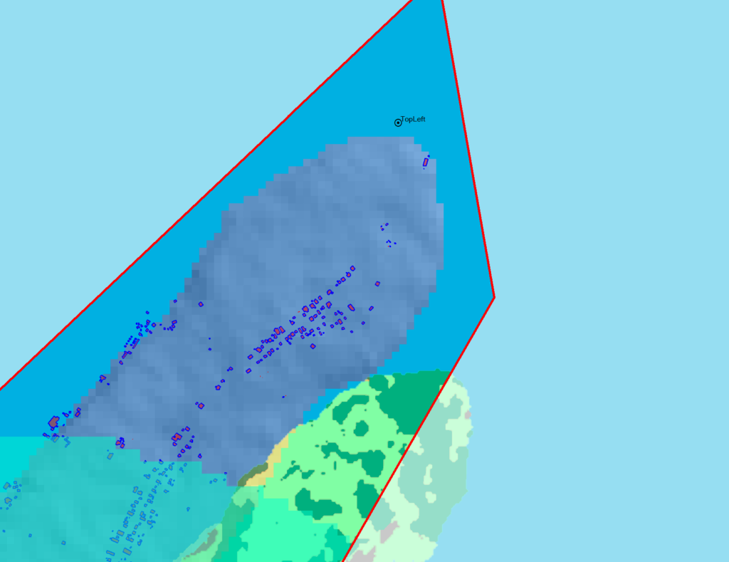
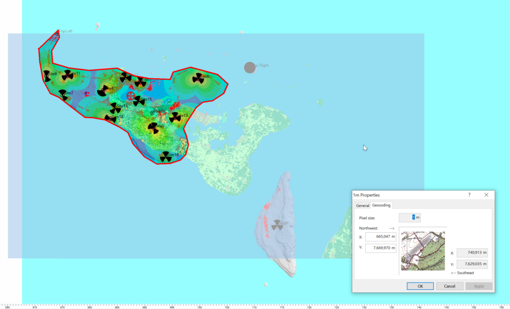
Then – and stick with me, this is very technical – I mess with the values until the maps line up into the correct position. Increase X, decrease Y, dialing it it in until the clutter map lines up with the other maps I’ve got.
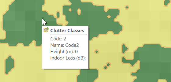
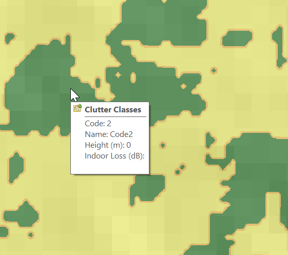
Right, now we’ve got the data but we don’t have any values.
Each color represents a clutter class, but we haven’t set any actual height or losses for that material.
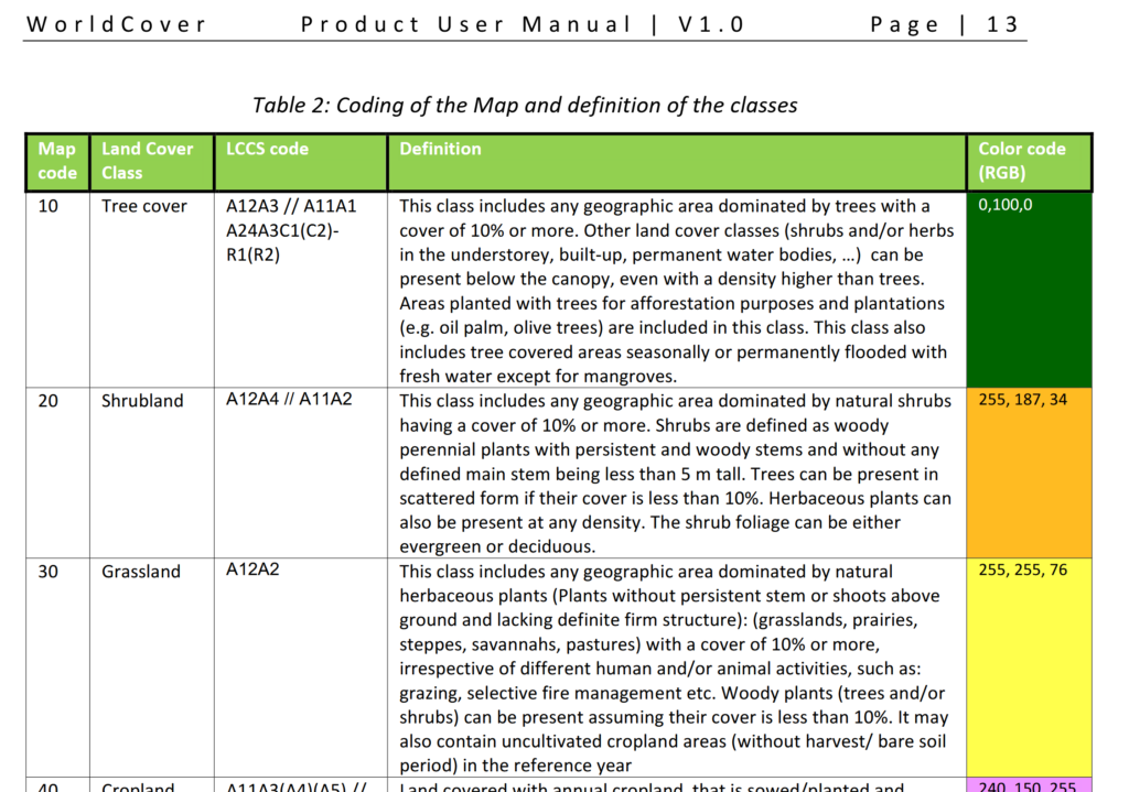
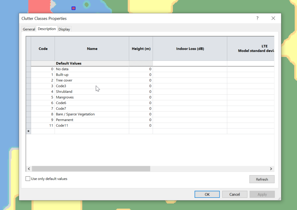
Alas the Map Code does not match with the table in the manual, but the colours do, here’s what mine map to:
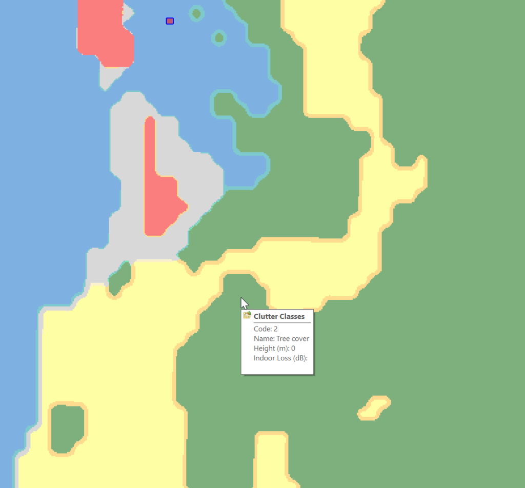
Which means when hovering over a layer of clutter I can see the type:
Next we need to populate the heights, indoor and outdoor losses for that given clutter. This is a little more tricky as it’s going to vary geography to geography, but there’s indicative loss numbers available online pretty easily.
Once you’ve got that plugged in you can run your predictions and off you go!
Concrete, steel and labor are some of the biggest costs in building a cell site, and yet all the focus on cost savings for cell sites seems to focus on the RAN, but the actual RAN equipment isn’t all that much when you put it into context.
I think this is mostly because there aren’t folks at MWC promoting concrete each year.
But while I can’t provide any fancy tricks to make towers stronger or need less concrete for foundations, there’s some potential low-hanging fruit in terms of installation of sites that could save time (and therefor cost) during network refreshes.
I don’t think many folks managing the RAN roll-outs for MNOs have actually spent a week with a tower crew rolling this stuff out. It’s hard work but a lot of it could be done more efficiently if those writing the MOPs and deciding on the processes had more experience in the field.
Disclaimer: I’m primarily a core networks person, this is the job done from a comfy chair. This is just some observations from the bits of work I’ve done in the field building RAN.
Standardize Power Connectors
Currently radio units from the biggest RAN vendors (Ericsson, Nokia, Huawei, ZTE & Samsung) each use different DC power connectors.
This means if you’re swapping from one of these vendors to another as part of a refresh, you need new power connectors.
If you’re lucky you’re able to reuse the existing DC power cables on the tower, but that means you’re up on a tower trying to re-terminate a cable which is a fiddly job to do on the ground, and far worse in the air. Or if you’re unlucky you don’t have enough spare distance on the DC cables to do the job, then you’re hauling new DC cables up a tower (and using more cables too).
While Huawei and ZTE have adopted for push connectors with the raw cables behind a little waterproof door.
If we could just settle on one approach (either is fine) this could save hours of install time on each cell site, extrapolate that across thousands of cell sites for each network, and this is a potentially large saving.
Standardize Fiber Cables
The same goes for waterproofing fibre, Ericsson has a boot kit that gets assembled inline over the connectors, Nokia has this too, as well as a rubber slide over cover boot on pre-term cables.
Again, the cost is fairly minimal, but the time to swap is not. If we could standardize a break out box format on the top of the tower and a LC waterproofing standard, we could save significant time during installs, and as long as you over-provision the breakout (The cost difference between a 6 core fiber vs a 48 core fibre is a few dollars), you can save significant time having to rerun cables.
Yes, we’ve all got horror stories about someone over-bending fiber, and if you reused fibre between hardware refresh cycles, but modern fiber is crazy tough so the chances of damaging the reused fiber is pretty slim, and spare pairs are always a good thing.
Preterm DC Cables
Every cell site install features some poor person squatting on the floor (if they’re savvy they’ve got a camping stool or gardening kneeling mat) with a “gut buster” crimping tool swaging on connectors for the DC lugs.
If we just used the same lugs / connectors for all the DC kit inside the cell sites, we could have premade DC cables in various lengths (like everyone does with Ethernet cables now), rather than making each and every cable off a spool (even if it is a good ab workout).
I dunno, I’m just some Core network person who looks at how long all this takes and wonders if there’s a way it could be done better, am I crazy?
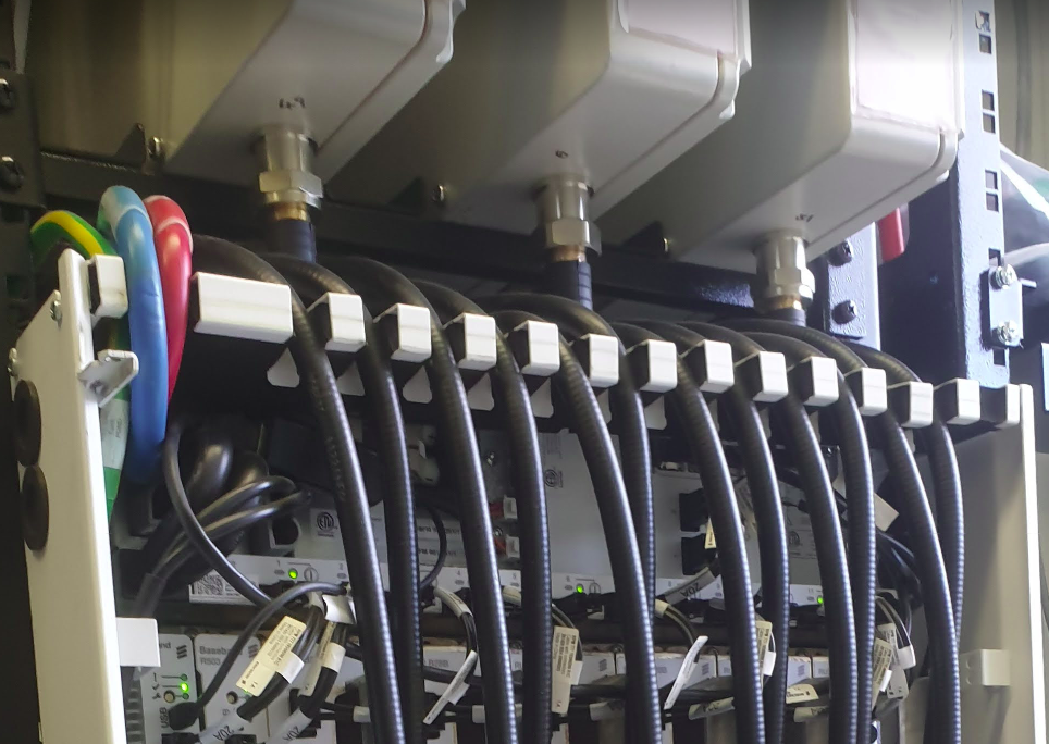
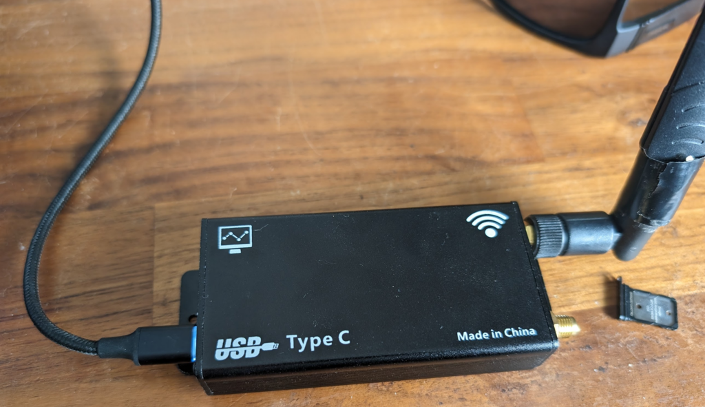
Last year we deployed some Hughes HL1120W OneWeb terminals in one of the remote cellular networks we support.
Unfortunately it was failing to meet our expectations in terms of performance and reliability – We were seeing multiple dropouts every few hours, for between 30 seconds and ~3 minutes at a time, and while our reseller was great, we weren’t really getting anywhere with Eutelsat in terms of understanding why it wasn’t working.
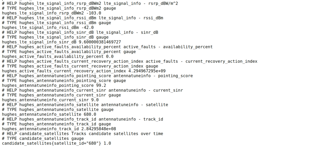
Luckily for us, Hughes (who manufacture the OneWeb terminals) have an unprotected API (*facepalm*) from which we can scrape all the information about what the terminal sees.
As that data is in an API we have to query, I knocked up a quick Python script to poll the API and convert the data from the API into Prometheus data so we could put it into Grafana and visualise what’s going on with the terminals and the constellation.
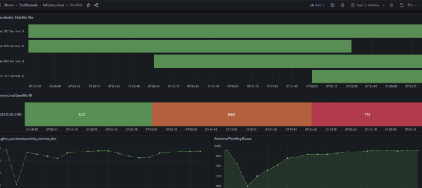
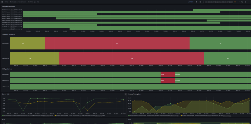
After getting all this into Grafana and combining it with the ICMP Blackbox exporter (we configured Blackbox to send HTTP requests and ICMP pings out of each of the different satellite terminals we had (a mix of OneWeb and others)) we could see a pattern emerging where certain “birds” (satellites) that passed overhead would come with packet loss and dropouts.
It was the same satellites each time that led to the drops, which allowed us to pinpoint to say when we see this satellite coming over the horizon, we know there’s going to be some packet loss.
In the end Eutelsat acknowledged they had two faulty satellites in the orbit we are using, hence seeing the dropouts, and they are currently working on resolving this (but that actually does require rockets, so we’re left without a usable service for the time being) but it was a fun problem to diagnose and a good chance to learn more about space.
Packet loss on the two OneWeb terminals (Not seen on other constellation) correlated with a given satellite pass
The repo has instructions for use and the Grafana templates we used.
At one point I started playing with the OneWeb Ephemeris data so I could calculate the azimuth and elevation of each of the birds from our relative position, and work out distances and angles from the terminal. The maths was kinda fun, but oddly the datetimes in the OneWeb ephemeris data set seems to be about 10 years and 10 days behind the current datetime – Possibly this gives an insight into OneWeb’s two day outage at the start of the year due to their software not handling leap years.
Despite all these teething issues I’m still optimistic about OneWeb, Kupler and Qianfan (Thousand Sails) opening up the LEO market and covering more people in more places.
Update: Thanks to Scott via email who sent this: One note, there’s a difference between GPS time and Unix time of about 10 years 5 days. This is due to a) the Unix epoch starting 1970-01-01 and the gps epoch starting 1980-01-05 and b) gps time is not adjusted for leap seconds, and ends up being offset by an integer number of seconds.
Technology is constantly evolving, new research papers are published every day.
But recently I was shocked to discover I’d missed a critical development in communications, that upended Shannon’s “A mathematical theory of communication”.
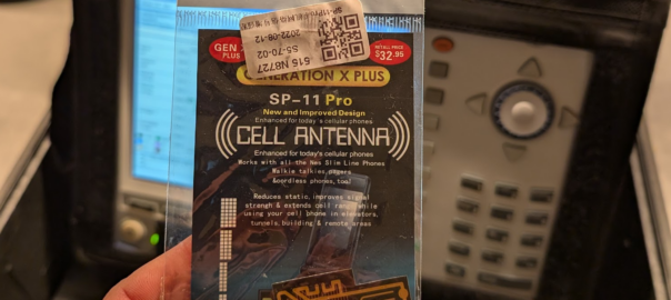
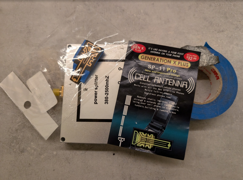
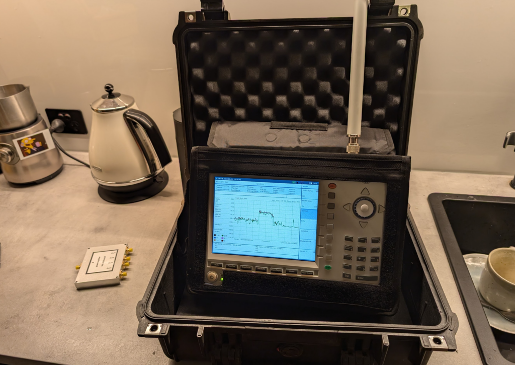
I’m talking of course, about the GENERATION X PLUS SP-11 PRO CELL ANTENNA.
I’ve been doing telecom work for a long time, while I mostly write here about Core & IMS, I am a licenced rigger, I’ve bolted a few things to towers and built my fair share of mobile coverage over the years, which is why I found this development so astounding.
With this, existing antennas can be extended, mobile phone antennas, walkie talkies and cordless phones can all benefit from the improvement of this small adhesive sticker, which is “Like having a four foot antenna on your phone”.
So for the bargain price of $32.95 (Or $2 on AliExpress) I secured myself this amazing technology and couldn’t wait to quantify it’s performance.
Think of the applications – We could put these stickers on 6 ft panel antennas and they’d become 10ft panels. This would have a huge effect on new site builds, minimize wind loading, less need for tower strengthening, more room for collocation on the towers due to smaller equipment footprint.
Luckily I have access to some fancy test equipment to really understand exactly how revolutionary this is.
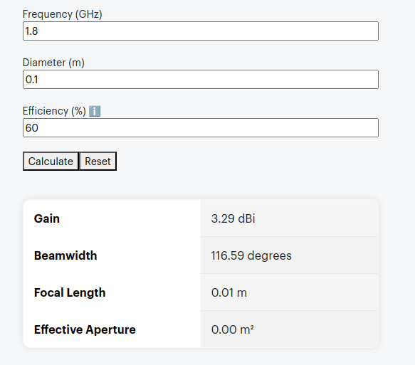
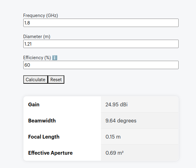
The packaging says it’s like having a 4 foot antenna on your phone, let’s do some very simple calculations, let’s assume the antenna in the phone is currently 10cm, and that with this it will improve to be 121cm (four feet).
Projected Gain (Post Sticker)Formulas Used
According to some basic projections we should see ~21dB gain by adding the sticker, that’s a 146x increase in performance!
Man am I excited to see this in action.
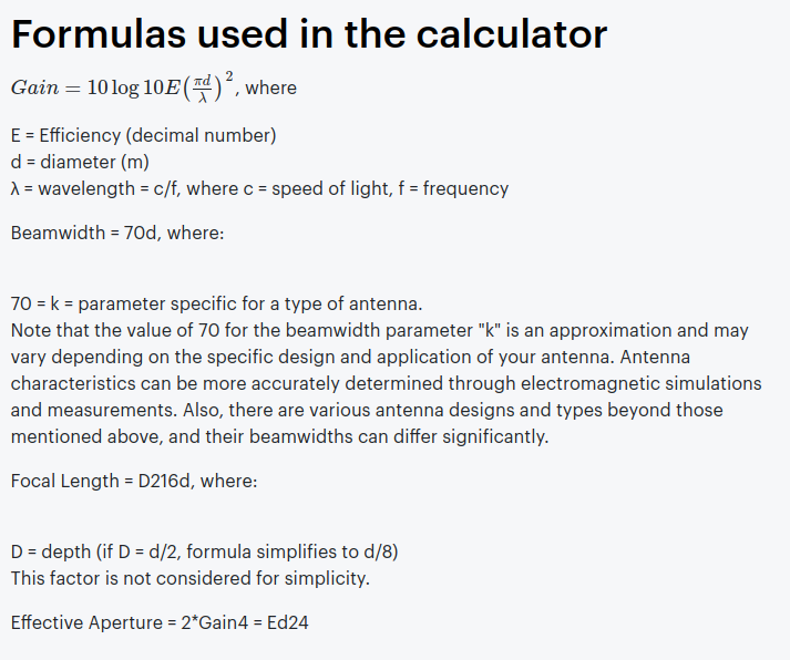
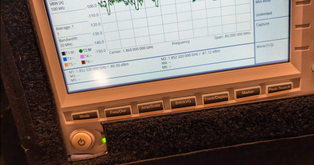
Fortunately I have access to some fun cellular test equipment, including the Viavi CellAdvisor and an environmentally controlled lab my kitchen bench.
I put up a 1800Mhz (band 3) LTE carrier in my office in the other room as a reference and placed the test equipment into the test jig (between the sink and the kettle).
We then took baseline readings from the omni shown in the pictures, to get a reading on the power levels before adding the sticker.
We are reading exactly -80dBm without the sticker in place, so we expertly put some masking tape on the omni (so we could peel it off) and applied the sticker antenna to the tape on the omni antenna.
At -80dBm before, by adding the 21dB of gain, we should be put just under -60dBm, these Viavi units are solid, but I was fearful of potentially overloading the receive end from the gain, after a long discussion we agreed at these levels it was unlikely to blow the unit, so no in-line attenuation was used.
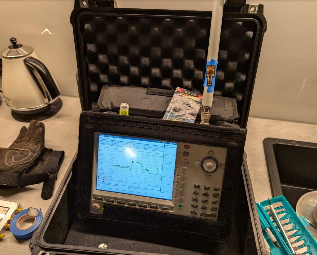
Okay, </sarcasm> I was genuinely a little surprised by what we found; there was some gain, as shown in the screenshot below.
Marker 1 was our reference without the sticker, while reference 2 was our marker with the sticker, that’s a 1.12dB gain with the sticker in place. In linear terms that’s a ~30% increase in signal strength.
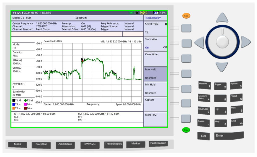
Screenshot
So does this magic sticker work? Well, kinda, in as much that holding onto the Omni changes the characteristics, as would wrapping a few turns of wire around it, putting it in the kettle or wrapping it in aluminum foil. Anything you do to an antenna to change it is going to cause minor changes in characteristic behavior, and generally if you’re getting better at one frequency, you get worse at another, so the small gain on band 3 may also lead to a small loss on band 1, or something similar.
So what to make of all this? Maybe this difference is an artifact from moving the unit to make a cup of tea, the tape we applied or just a jump in the LTE carrier, or maybe the performance of this sticker is amazing after all…
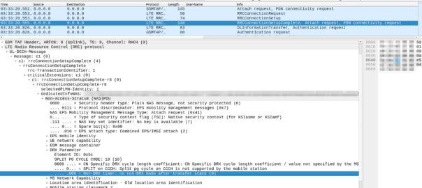
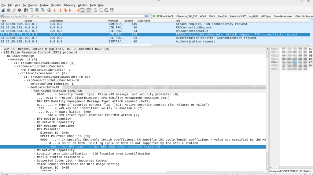
Recently we were on a project and our RAN guy was seeing UEs hand between one layer and another over and over. The hysteresis and handover parameters seemed correct, but we needed a way to see what was going on, what the eNB was actually advertising and what the UE was sending back.
In a past life I had access to expensive complicated dedicated tooling that could view this information transmitted by the eNB, but now, all I need is a cellphone or a modem with a Qualcomm chip.
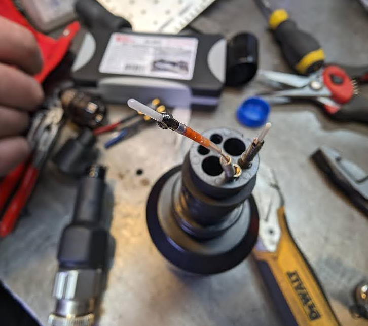
I came across these the other day, they’re DC & Fibre in the same connector body.
Rather than breaking out to a fibre and an Anderson connector, you’ve got both in one connector, with provision for an extra fibre pair too, then on the other end this splits into the RRU power connector, used by Ericsson and Nokia, and a LC connector for the fibre into the RRU.
I pulled it all apart this to see how it fitted together, it looks like they’re factory pre-term cables, rather than being spliced to length, which I guess makes sense. Cool design!
Up close view of the connectorDC breaks out when you pull it apartAnd the fibres are held in with springs to the top half of the connector bodyAnd the breakout to LC and RRU DC connectors
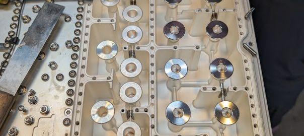
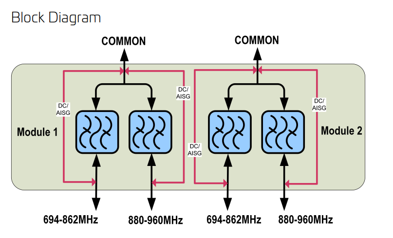
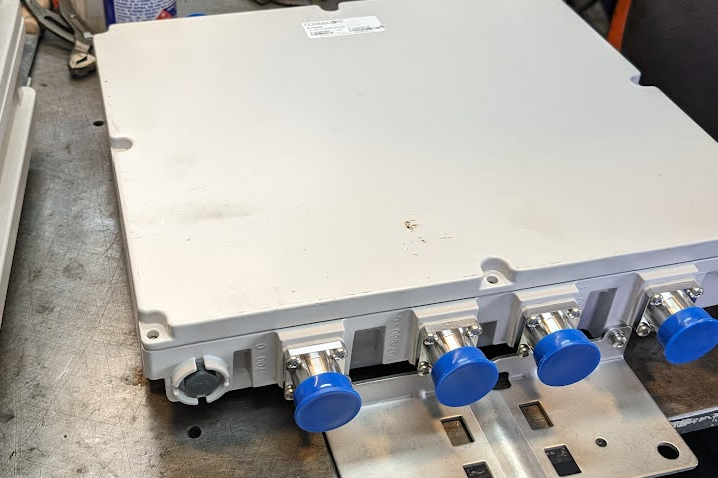
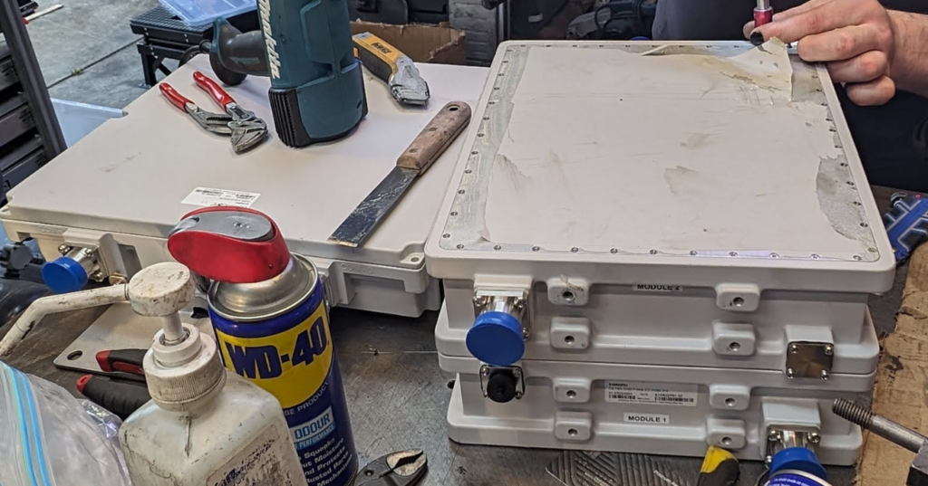
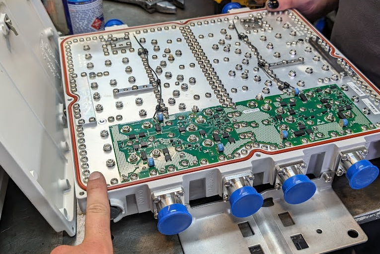
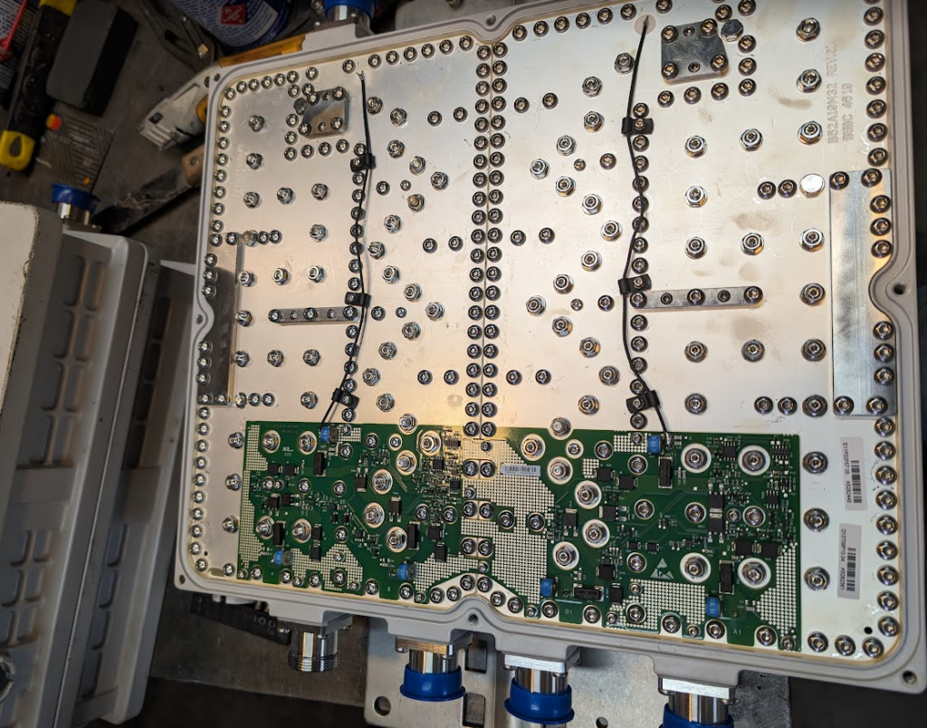
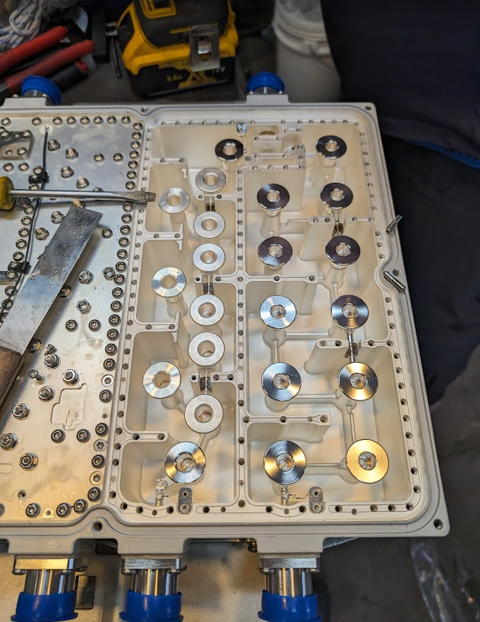
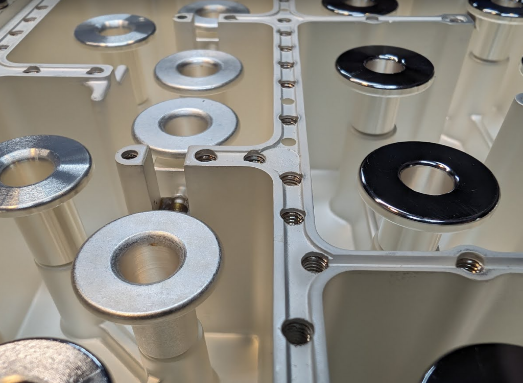
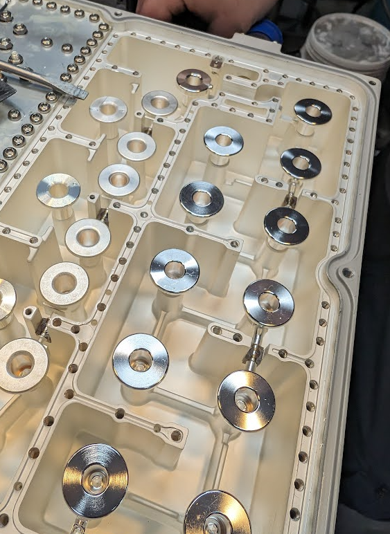
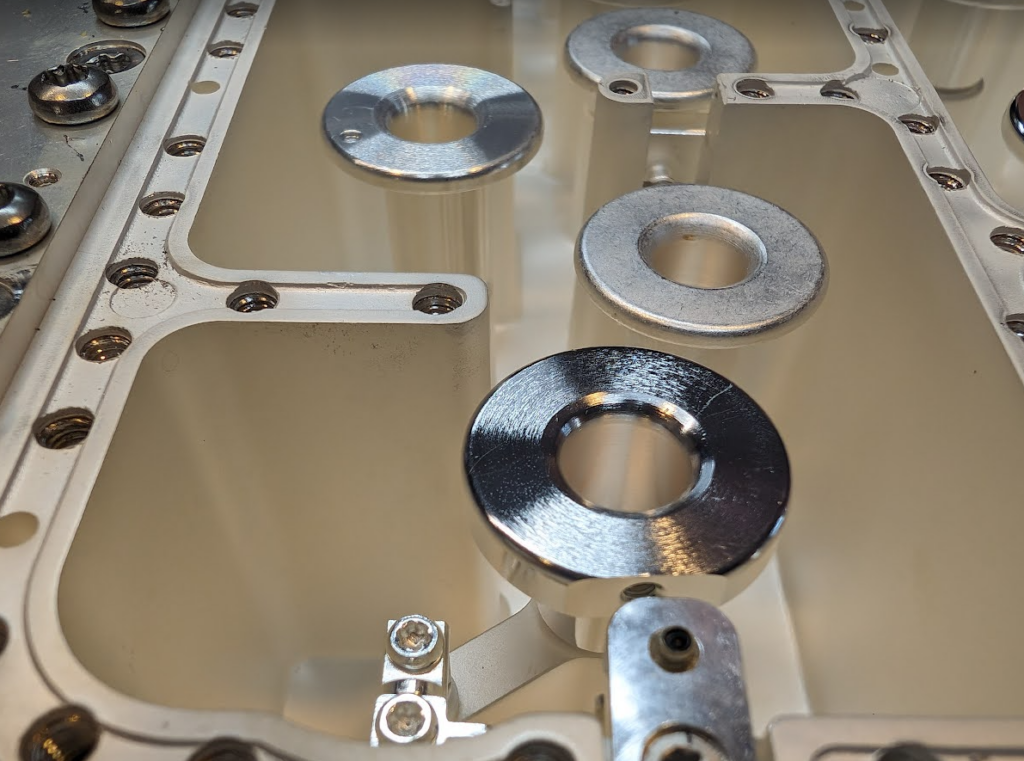
I recently ended up with a few Commscope RF combiners from a cell site, they’re not on frequencies that are of any use to us, so, let’s see what’s inside.
The units on the bench are Commscope Diplexer units, these ones allow you to put a signal between 694-862Mhz, and another signal between 880-960Mhz, on the same RF feeder up the tower.
It’s a nifty trick from the days where radio units lived at the bottom of the tower, but now with Remote Radio Units, and Active Antenna Units, it’s becoming increasingly uncommon to have radio units in the site hut, and more common to just run DC & fibre up the tower and power a radio unit right next to the antenna – This is especially important for higher frequencies where of course the feeder loss is greater.
Diplexer unit before it is maimed…
Anywho, that’s about all I know of them, after the liberal application of chemicals to remove the stickers and several burns from a heat gun, we started to get the unit open, to show the zillion adjustment bolts, and finely machined parts.
A lot of screwsBonus TMA
Thanks to Oliver for offering up the bench space when I rocked to up to their house with some stuff to pull apart.
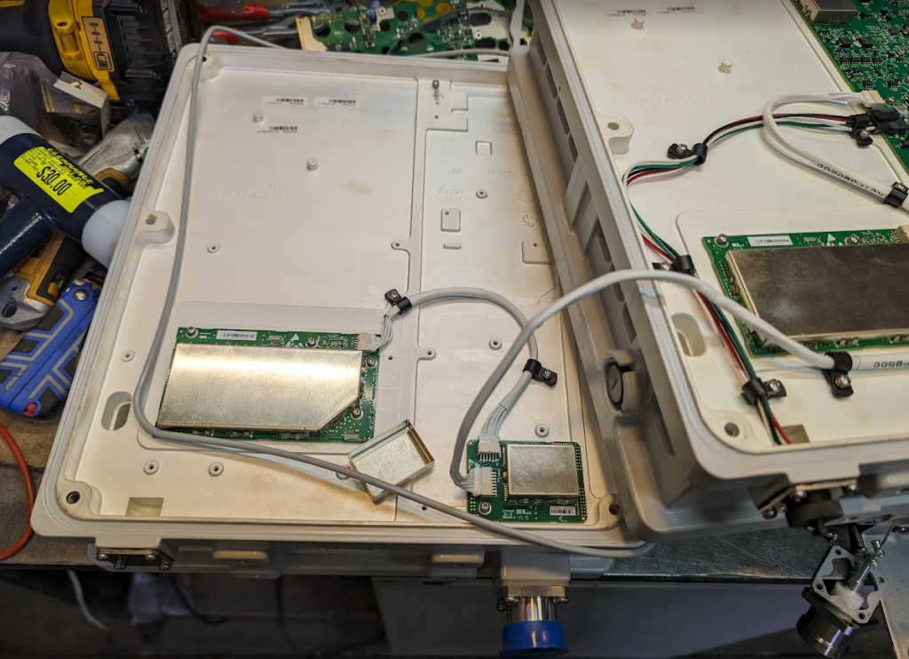
Last year I purchased a cheap second hand Huawei macro base station – there’s lots of these on the market at the moment due to the fact they’re being replaced in many countries.
I’m using it in my lab environment, and as such the config I’ve got is very “bare bones” and basic. Keep in mind if you’re looking to deploy a Macro eNodeB in production, you may need more than just a blog post to get everything tuned and functioning properly…
In this post we’ll cover setting up a Huawei BTS3900 eNodeB from scratch, using the MML interface, without relying on the U2020 management tool.
Obviously the details I setup (IP Addressing, PLMN and RF parameters) are going to be different to what you’re configuring, so keep that in mind, where I’ve got my MME Addresses, site IDs, TACs, IP Addresses, RFUs, etc, you’ll need to substitute your own values.
A word on Cabinets
Typically these eNodeBs are shipped in cabinets, that contain the power supplies, alarm / environmental monitoring, power distribution, etc.
Early on in the setup process we’ll be setting the cabinet types we’ve got, and then later on we’ll tell the system what we have installed in which slots.
This is fine if you have a cabinet and know the type, but in my case at least I don’t have a cabinet manufactured by Huawei, just a rack with some kit mounted in it.
This is OK, but it leads to a few gotchas I need to add a cabinet (even though it doesn’t physically exist) and when I setup my RRUs I need to define what cabinet, slot and subrack it’s in, even though it isn’t in any. Keep this in mind as we go along and define the position of the equipment, that if you’re not using a real-world cabinet, the values mean nothing, but need to be kept consistent.
To begin we’ll need to setup the basics, by disabling DHCP and setting an local IP Address for the unit.
 SET DHCPSW: SWITCH=DISABLE;
 SET LOCALIP: IP="192.168.5.234", MASK="255.255.248.0";
Obviously your IP address details will be different. Next we’ll add an eNodeB function, the LMPT / UMPT can have multiple functions and multiple eNodeBs hosted on the same hardware, but in our case we’re just going to configure one:
Again, your eNodeB ID, location, site name, etc, are all going to be different, as will your location.
Next we’ll set the system to maintenance mode (MNTMODE), so we can make changes on the fly (this takes the eNB off the air, but we’re already off the air), you’ll need to adjust the start and end times to reflect the current time for the start time, and end time to be after you’re done setting all this up.
SET MNTMODE: MNTMode=INSTALL, ST=2013&09&20&15&00&00, ET=2013&09&25&15&00&00, MMSetRemark="NewSite Install";
Next we’ll set the operator details, this is the PLMN of the eNodeB, and create a new tracking area.
Next we’ll be setting and populating the cabinets I mentioned earlier. I’ll be telling the unit it’s inside a APM30 (Cabinet 0), and in Cabinet Number 0, Subrack 0, is a BBU3900.
 //To modify the cabinet type, run the following command:
 ADD CABINET:CN=0,TYPE=APM30;
 //Add a BBU3900 subrack, run the following command:
 ADD SUBRACK:CN=0,SRN=0,TYPE=BBU3900;
 //To configure boards and RF datas, run the following commands:
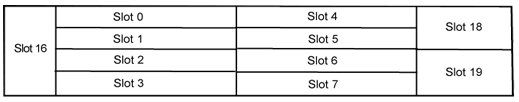
And inside the BBU3900 there’s some cards of course, and each card has as slot, as per the drawing below.
In my environment I’ve got a LMPT in slot 7, and a LBBP in Slot 3. There’s a fan and a UPEU too, so: We’ll add a board in Slot No. 7, of type LMPT, We’ll add a board in Slot No. 3, of type LBBP working on FDD, We’ll add a fan board in Slot No. 16, and a UPEU in Slot No. 18.
Huawei publish design guides for which cards should be in which slots, the general rule is that your LMPT / UMPT card goes in Slot 7, with your BBP cards (UBBP or LBBP) in slots 3, then 2, then 1, then 0. Fans and UPEUs can only go in the slots designed to fit them, so that makes it a bit easier.
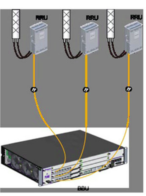
Next we’ll need to setup our RRUs, for this we’ll need to setup an RRU chain, which is the Huawei term for the CPRI links and add an RRU into it:
//Modify the reference signal power.
MOD PDSCHCFG: LocalCellId=1, ReferenceSignalPwr=-81;

//Add an operator for the cell.
ADD CELLOP: LocalCellId=0, TrackingAreaId=0;

//Activate the cell.
ACT CELL: LocalCellId=1;
For the past few months I’ve had a Band 78 NR active antenna unit sitting next to my desk.
It’s a very cool bit of kit that doesn’t get enough love, but I thought I’d pop open the radome and take a peek inside.
Individual antenna elements
What I found very interesting is that it’s not all antennas in there!
… 29, 30, 31, 32. Yup. Checks out.
There are the expected number of antennas (I mean if I opened it up and found 31 antennas I’d have been surprised) but they don’t take up the whole volume of the unit, only about half,
AAU with Radome reinstalled
Well, after that strip show, back to sitting in my office until I need to test something 5G SA again…
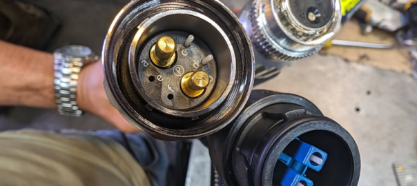
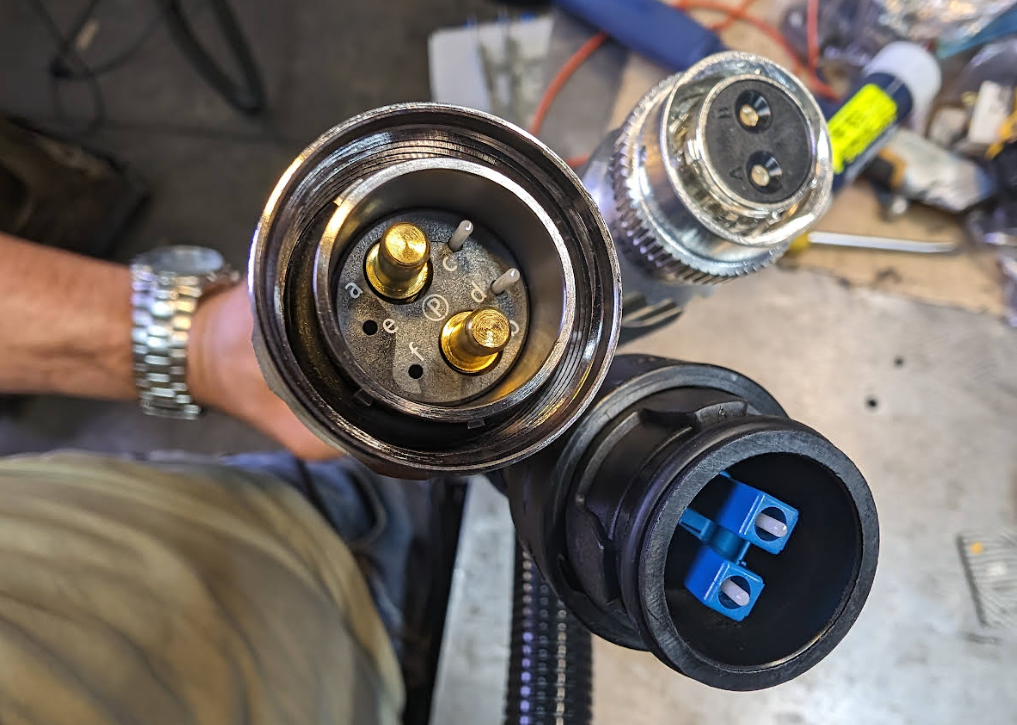
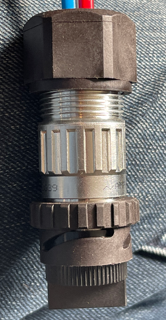
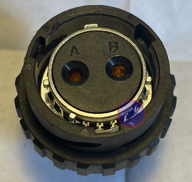
Something that’s kind of great is that the current generation of Ericsson RRUs and Nokia RRUs, use the same power connector – The Amphenol “Amphe-OBTS” series connector.
Construction and wiring of these connectors is the same for both, and with one little trick, we can use the connector for both Ericsson and Nokia RRUs (Airscale and later).
This pin that stops the connector from being “universal” but is easily removed.
The connectors are not quite universal, in order to use it in both you need to knock off a small pin on the connector, I’d suggest doing this before you assemble it, put the connector on it’s back, facing upwards, and hit this with a screwdriver / chisel and it’ll pop off with very little effort.
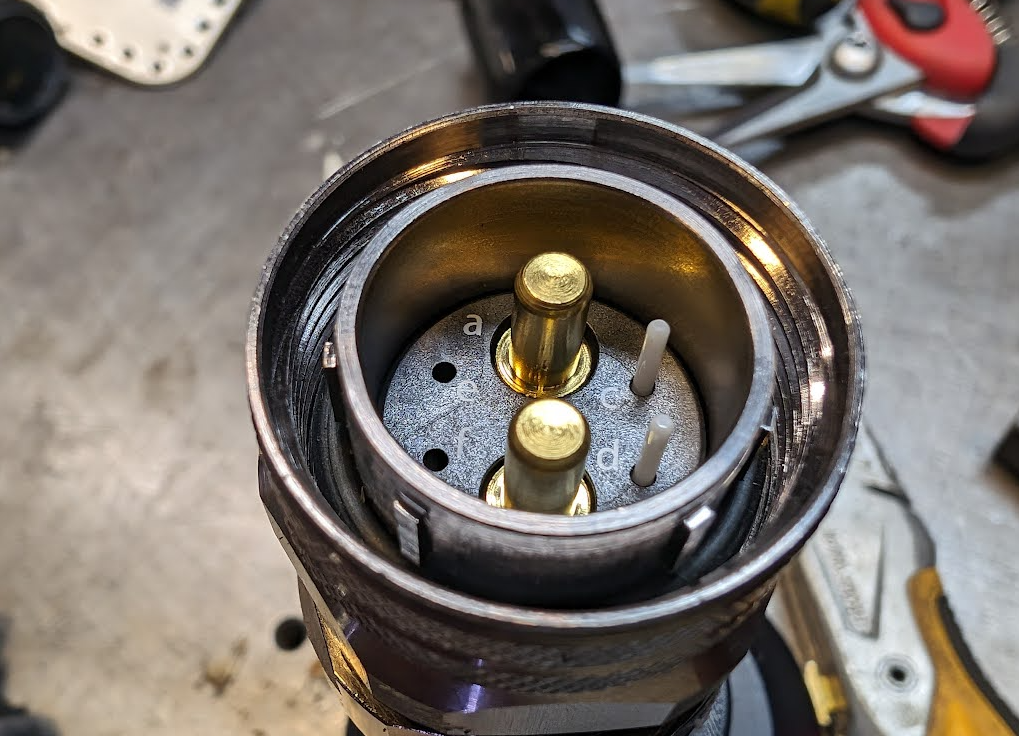
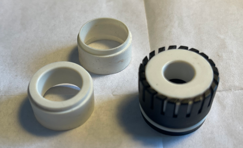
Assembling the connectors starts by working out the diameter of the grommet you need to fit your cable, the connector comes with the grommet for 9-14mm, but in the bag you’ll usually get grommets for 6-9mm cable and 14-18mm cable.
Grab the correct one for your cable diameter, and pop into the black fingered cage (‘gland adapter’) shown in the bottom right of the below photo.
Grommets and gland adapter
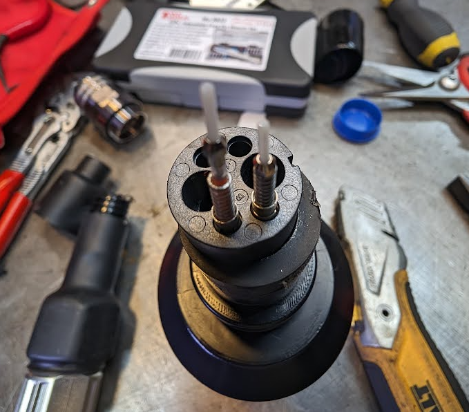
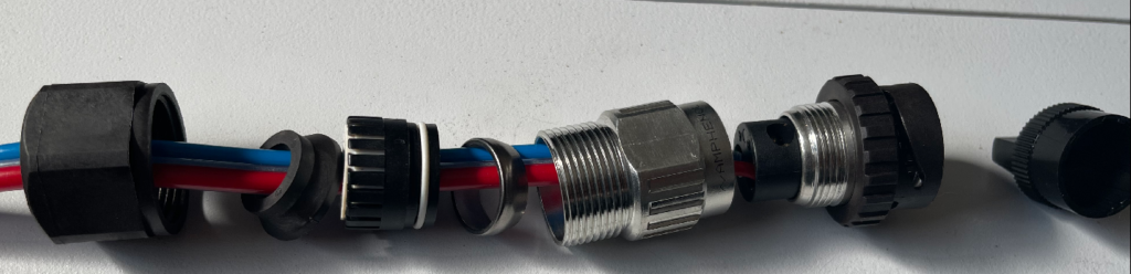
Next we line all the parts up along the cable and screw it all together:
The end-cap is actually very useful for stopping the female end of the connector from spinning when you’re assembling the cable, so don’t throw it away!
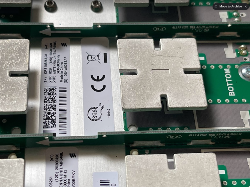
I recently had a bunch of antennas profiles in .msi format, which is the Planet format for storing antenna radiation patterns, but I’m working in Forsk Atoll, so I needed to convert them,
To load these into Atoll, you need to create a .txt file with each of the MSI files in each of the directories, I could do this by hand, but instead I put together a simple Python script you point at the folder full of your MSI files, and it creates the index .txt file containing a list of files, with the directory name.txt, just replace path with the path to your folder full of MSI files,
#Atoll Index Generator
import os
path = "C:\Users\Nick\Desktop\Antennas\ODV-065R15E-G"
antenna_folder = path.split('\\')[-1]
f = open(path + '\\' + 'index_' + str(antenna_folder) + '.txt', 'w+')
files = os.listdir(path)
for individual_file in files:
    if individual_file[-4:] == ".msi":
        print(individual_file)
        f.write(individual_file + "\n")

f.close()
How do humans talk to base stations? For Huawei at least the answer to this is through MML – Man-Machine-Language,
It’s command-response based, which is a throwback to my Nortel days (DMS100 anyone?),
So we’re not configuring everything through a series of parameters broken up into sections with config, it’s more statements to the BTS along the lines of “I want you to show me this”, or “Please add that” or “Remove this bit”,
The instruction starts of with an operation word, telling the BTS what we want to do, there’s a lot of them, but some common examples are; DSP (Display), LST (List), SET (Set), MOD (Modify) and ADD (Add).
After the operation word we’ve got the command word, to tell the BTS on what part we want to execute this command,
A nice simple example would be to list the software version that’s running on the BTS. For this we’d run
LST SOFTWARE:;
And press F9 to execute, which will return a list of software on the BTS and show it in the terminal.
Note at the end the :; – the : (colon) denotes the end of a command word, and after it comes the paratmeters for the command, and then the command ends with the ; (semi-colon). We’ll need to put this after every command.
Let’s look at one more example, and then we’ll roll up our sleves and get started.
Note: I’m trying out GIFs to share screen recordings instead of screenshots. Please let me know if you’re having issues with them.
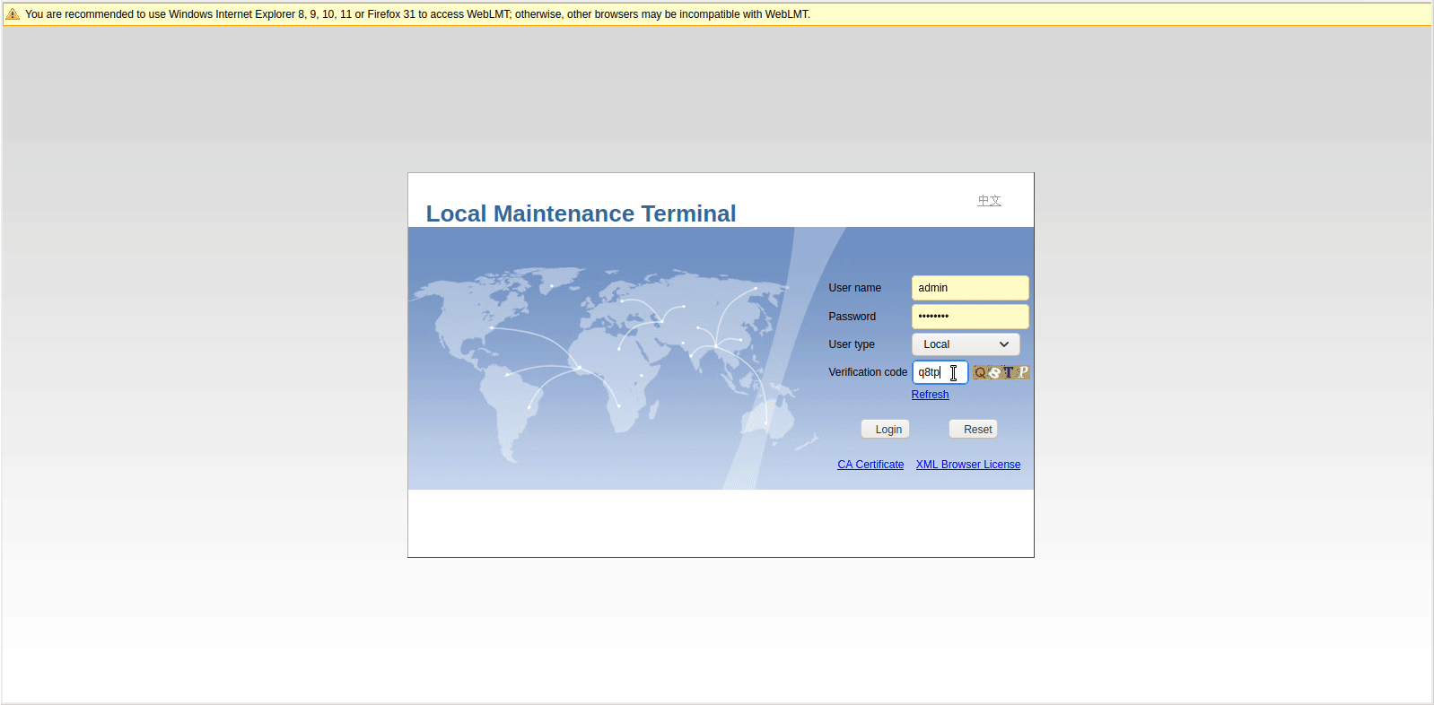
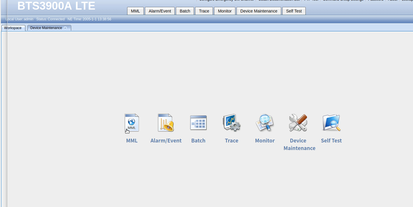
So once you’ve logged into WebLMT, selecting MML is where we’ll do all our config, let’s log in and list the running applications.
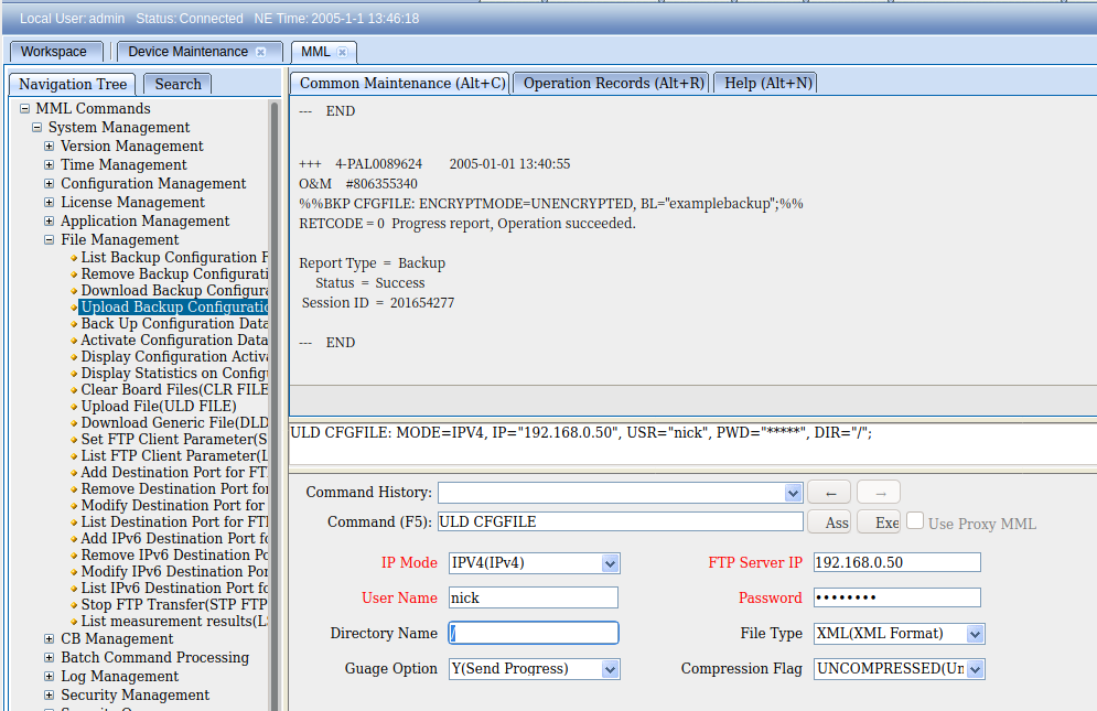
So far we’ve only got some fairly basic data, listing and displaying values, so let’s try something a bit more complex, taking a backup of the config, in encrypted mode, with the backup label “blogexamplebackup”,
If you’ve made it this far there’s a good chance you’re thinking there’s no way you can remember all these commands and parameters – But I’ve got some good news, we don’t really need to remember anything, there’s a form for this!
And if we want to upload the backup file to an FTP server, we can do this as well, in the navigation tree we find Upload Backup Configuration, fill in the fields and click the Exec button to execute the command, or press F9.
These forms, combined with a healthy dose of the search tab, allow us to view and configure our BTS.
I’ve still got a lot to learn about getting end-to-end configuration in place, but this seems like a good place to start,
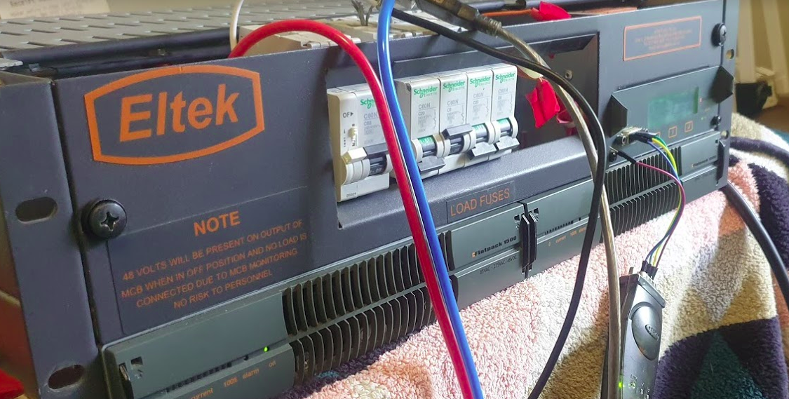
All the gear I’ve got so far for my DIY RAN Project requires -48vDC to power it up.
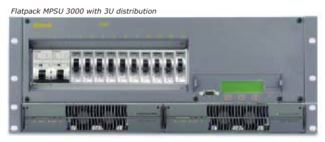
Back to online auction websites and preso I’ve ended up with an Eltek MPSU3000, from the mid 2000s.
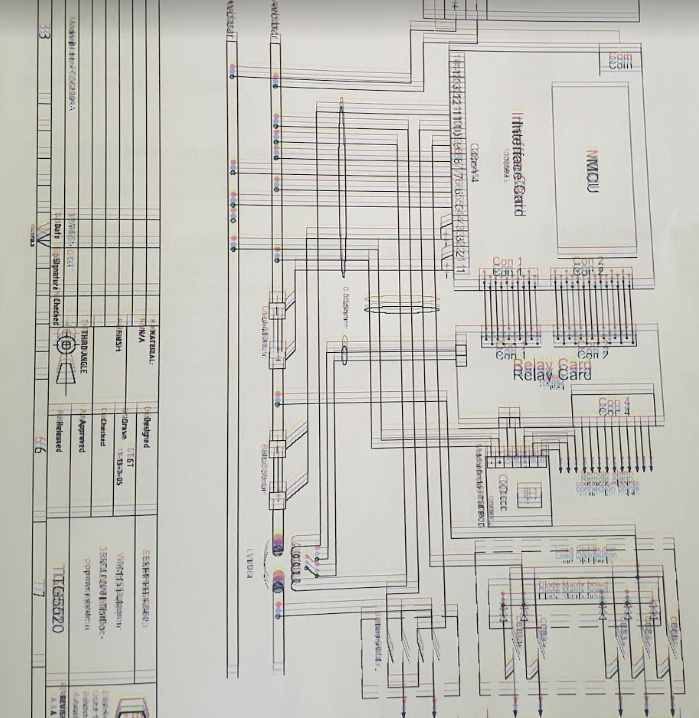
The fellow I bought it from was even nice enough to throw a binder full of printed documentation, which included a full circuit layout diagram, however this was obviously in the days of old school printers, and each of the colours were offset, providing a literal headache when reading and a bit of a reminder of what printed documents were like to deal with…
I get a headache just looking at the colours in this…
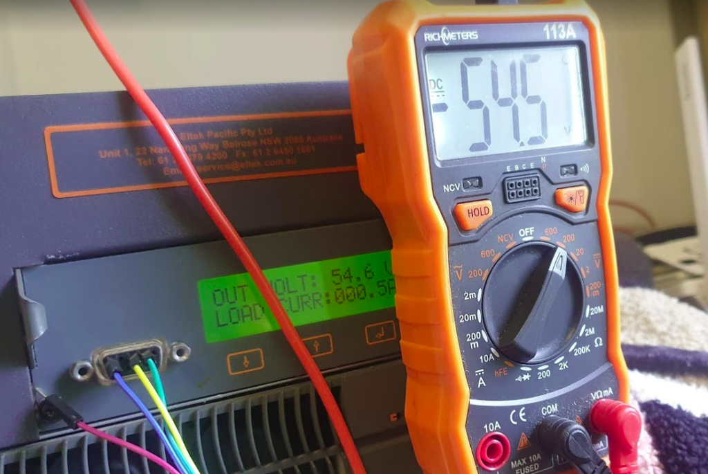
So after a bit of tinkering, wiring and reconnecting the temperature probe, I managed to fire the unit up,
While it complained about the absence of batteries (As well as rectifying AC to DC it manages and maintains banks of batteries to provide a backup power supply), it worked, and provided a very stable, clean -54v DC.
I’ve got a very old (1948) Ring Generator / Ring Machine, (same as this one) so I wired it into the rectifier and it came to life, drawing 3 amps in the process.
The Huawei gear uses proprietary power connectors, I’ve managed to start it using crocodile clips and good luck to get it powered up, but I’ve got to work out a more permanent solution before I can rack all the gear and have it setup properly.
The Eltek rectifier has a number of relay contacts in the unit that can be programed to trigger in different conditions, ie mains power lost, battery fault, over temperature, etc.
These relay contacts are then wired into some sort of alarm input, to share alarm state with external monitoring equipment. (Modern rectifiers just have Ethernet and connect over TCP/IP, but this one just has a serial port and an AT command set for connecting it to a dialup modem.)
The BTS3900 has the Universal Power and Environment Unit (UPEU), which allows me to connect external alarm inputs, for things like this, water sensors, smoke detectors and intruder alarms, so hopefully I’ll get that in place when I’m further down the line.
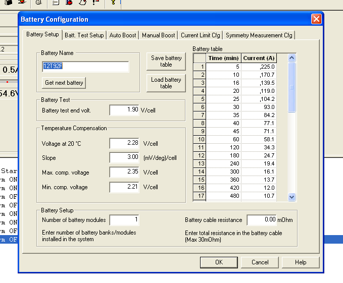
But to program these requires the software, which I couldn’t find anywhere online. As a last ditch attempt I reached out to the manufacturer, Eltek, and asked if they’d be so kind as to send me a copy. I wasn’t expecting much, but the next day, they sent me back all the manuals and the software the next day, for a 15 year old, long surpassed product. Very impressed!
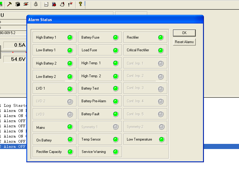
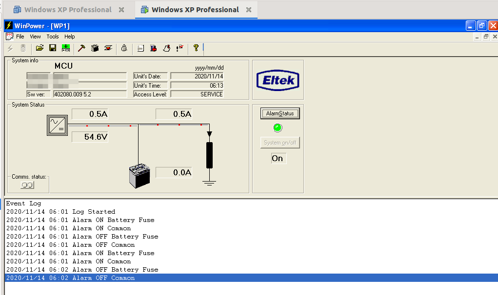
So with the aid of VMware, Windows XP, USB-Serial adapters and jumper wires, I managed to connect to the Rectifier Controller with the software and had a poke around.
Pretty impressive functionality for something this old, but no ability to monitor if MCBs have been tripped or remotely power off/on outputs.
While the unit can do some very clever things with battery management, for my lab setup I can’t see myself going to the effort of adding batteries. So for now the Rectifier’s just converting AC mains into -48vDC, but I may string some batteries in the future.
For anyone who’s ended up here looking for info on these units, or the first generation Eltek Flatpacks, I’ve attached some documentation below. The software isn’t readily available online, so I won’t post it here, but you can get it from Eltek directly.